MicroSurvey CAD can create and manipulate surfaces. A MicroSurvey CAD surface is the mathematical description of a surface which exactly honors all input data points. MicroSurvey CAD surfaces are a single-valued function of independent variables X and Y. This means that a surface only has one Z value for any given (X, Y), and so does not model overhanging surfaces or exactly vertical surfaces.

Surfaces may represent anything. Existing topography, proposed topography, thickness maps, geologic structure maps, sound decibels, magnetic readings, concentration distribution, slope maps, pressure gradient maps may all be represented as MicroSurvey CAD surfaces. MicroSurvey CAD has no limit on the number of points in a surface or the number of surfaces simultaneously used. The ultimate limitation is available space on your hard disk drive.

Surfaces contain one or more parts such as points, break lines, triangulated irregular networks (TIN), grids or triangulated grids (TGRD).

A surface is not an AutoCAD drawing entity, rather it is a mathematical description held in surface memory. Representations of a surface, such as points, contours, grids or TINs may be drawn into your drawing as point, line, polyline, 3D face, polyface mesh or mesh entities. It is important to keep the distinction between MicroSurvey CAD surfaces (which reside in surface memory (RAM)) and drawn entities representing parts of surfaces (which reside in the drawing database).

All drawing entities created by MicroSurvey CAD are placed in their proper position in 3D model space.

Surface memory

MicroSurvey CAD creates a unique unit of memory storage inside CAD-controlled memory commonly referred to as a surface.

Surface memory has the ability to manage an unlimited number of these surfaces (dependent on your machines resources). Multiple surfaces allow you to perform algebraic operations between different surfaces, resulting in surfaces representing thicknesses, cut and fill volumes, exaggerated surfaces, surfaces representing slopes and many other possibilities.

MicroSurvey CAD uses surface memory, rather than the CAD drawing database, to store and manipulate surfaces. Although surfaces are stored in CAD-controlled memory, a surface is not part of the drawing until you instruct MicroSurvey CAD to add it to the drawing by issuing a Draw response to a MicroSurvey CAD command such as Contour.

A surface will not be visible until you use specific display commands (Points, Breaks, Contour, TIN, Grid, Triangulated grid) and their Draw or Show options to either draw or temporarily display the surface in the current viewport or drawing. The Show option temporarily displays the requested contours or surface element on your drawing screen, until the next CAD Redraw. The Draw option adds the requested contours or surface element to the drawing database as CAD entities.

MicroSurvey CAD maintains one special surface which is the results surface named <.> “dot”. When you load point data into surface memory it can be placed into the <.> surface, or a named surface. The results of any surface operation are placed in the <.> surface. Any of these operations replace the pre-existing contents of the <.> surface. You may make copies of any surfaces or rename surfaces using the surface management commands within Surface Operations.

Surfaces in memory will not be saved when a CAD Save or End command is executed. MicroSurvey CAD instead provides a separate command (Write QSB) that allows the user to write a one or more surfaces to disk independently of the MicroSurvey CAD drawing. This provides more efficient use of storage (as much as 50% less) and preserves all parts of a surface in a quickly retrievable form. If you attempt to exit the MicroSurvey CAD program with surfaces still in memory, you will receive an alert and be offered the chance to save them. If you remain in the program and simply exit the drawing, you will not receive the same prompt, until you actually exit the program.

Parts of a Surface

The component parts of MicroSurvey CAD surfaces can be divided into data parts, which you supply, and calculated parts, which MicroSurvey CAD calculates. The following discussion of surface parts relates to the characteristics of the surface parts, not the methods used to create them. Realize that the elevations of calculated parts, such as a grid or triangulated grid, may be computed using different algorithms.

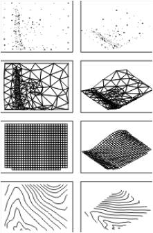
Basic parts of a surface

Data parts

The two main types of data MicroSurvey CAD uses to create surface models consist of point data and/or break lines.

Points

Menu: MsModeling | Extract from Drawing | Extract to Surface

Command: QSX

Icon:

Points form the basis of most surfaces. Points are unique X,Y,Z triplets in MicroSurvey CAD’s World Coordinate System. Point data may be loaded to surface memory by the following commands:

Extract to Surface (QSX)

Merge Extract (QSMX)

Read ASCII Points (QSL)

Read ASCII Table (QSML)

Read QSB File

Read DEM File

Active Coordinate Editor

The Extract commands extract point data from MicroSurvey CAD drawing entities (entities can include Points, Lines, Polylines, 3D Polylines, etc.). The Read commands read point data from disk files. The Active Coordinate Editor reads point data directly from point database files.

Breaks

Menu: MsModeling | Extract from Drawing | Extract Breaks

Command: QSBX

Icon:

Break line data (Breaks) are 3D polylines or 3D Lines which represent abrupt discontinuities in the slope of a surface (significant change in grade). Examples of breaks are the edges of ditches, walls, edge of pavement, road centerlines and curbs in surveying and civil engineering fields and faults in geology. Whereas a surface without breaks maintains continuous slope and curvature throughout, a surface with breaks may have abrupt changes in slope at the trace where the surface crosses break lines.

Break line data may be loaded to surface memory by the following commands:

Extract Breaks (QSBX)

Read ASCII Breaks (QSBL)

Read QSB File

The Extract Breaks command extracts break data from MicroSurvey CAD drawing entities such as 2D/3D polylines and 3D Lines. Read ASCII Breaks reads break data from disk files, such as survey data. Read QSB reads break data from MicroSurvey CAD surfaces previously stored to disk.

Calculated parts

The calculated parts of a surface are the Triangulated Irregular Network (TIN), Derivatives, Grid and Triangulated Grid (TGRD). Some MicroSurvey CAD commands calculate more than one of these parts.

Triangulated irregular network (TIN)

Menu: MsModeling | TIN Create / Edit | TIN

Command: TIN

Icon:

The triangulated irregular network, or TIN, is a three-dimensional model of a surface composed of planar triangular faces. MicroSurvey CAD generates it based on the Delauney criterion, by which points are connected optimally to make all triangles as nearly equilateral as possible. The TIN may be used directly for volumetrics, profiles, elevation analysis, contouring or as a surface to render. Since each vertex of the TIN is a surface point, a TIN honors all the points exactly.

MicroSurvey CAD also uses the TIN to identify neighboring points when calculating derivatives for gridded surfaces. MicroSurvey CAD can draw the TIN as lines, 3D faces or polyface mesh entities.

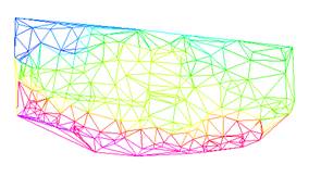
TIN created with MicroSurvey CAD

Derivatives

When MicroSurvey CAD generates a surface where surface curvature is calculated, slope information (1st and 2nd derivatives) are calculated at each vertex of the TIN, representing the slope of the surface at that vertex. The derivative order, weighting and blending parameters affecting this calculation are set within the MsModeling menu -> Configuration Settings -> Grid, dialog.

The 1st derivatives of a surface represent slope.

The 2nd derivatives of a surface represent curvature.

Whether or not surface curvature is calculated between control points is based on the Derivative setting in the Configuration Settings -> Grid dialog box. When surface curvature is requested, the derivatives are used to fit a smoothly curved polynomial surface to each triangular face of the TIN. By default this polynomial surface has continuous slope and curvature between all neighboring faces of the TIN, except at break lines, where the slopes are allowed to be different on either side of the break line. If a TIN is created from a data set including break lines, the break line information is totally represented in the resulting TIN and derivatives. The TIN, along with derivatives, represent the complete mathematical surface description. Both the Grid and TGRD commands use these to solve for elevation at each grid node during surface construction.

Input Data TIN without curvature

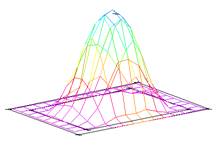
TGrid with curvature

Grid

Menu: MsModeling | Grid

Command: GRD

Icon:

The grid consists of a set of vertices, spaced rectangularly in the X and Y axes, with Z values conforming to the modeled surface. Although the mathematical model used honors the input data exactly, the resultant grid model is comprised of cells with vertices that are not members of the input point data set. Therefore, the final grid model will very nearly honor the input data set, but may not match the data set exactly. As a smaller grid cell size is used, any error between the input data set and the calculated grid is reduced. As a larger grid cell size is used, the potential error between the input data set and the calculated grid increases. The grid model provides for a smoother representation of the data, when contoured, than a TIN due to the larger number of vertices present for contour interpolation.

Gridding is very effective when dealing with data sets that do not contain break data. The grid does not have the capacity to truly represent break line data due to the fact that the cells have consistent spacing, causing the breaks to be smoothed to the grid cell size.

Data sets which contain break lines should be modeled with a TIN or TGRD, rather than a grid.

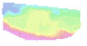
GRID created with MicroSurvey CAD

Triangulated Grid (TGRD)

Menu: MsModeling | Triangulated Grid

Command: TGRD

Icon:

The Triangulated Grid (TGRD) model combines the best parts of the TIN and grid models into one continuous model of a surface. The TGRD is used for surfaces which contain both point data and break line data, and produces a smooth curved surface away from break lines, but honors break lines exactly.

A Triangulated Grid consists of point data and densified 3D breakline data which have been internally gridded based on the derivative and cell size settings of Configuration Settings -> Grid dialog. The resulting grid node data, along with the breakline data, form a point set which is triangulated to form a special TIN termed a Triangulated Grid (TGRD). This TGRD is a TIN which honors breakline data exactly, but also may honor curvature data when away from breaklines.

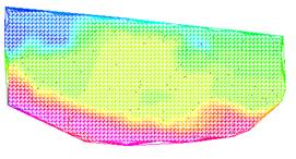
Triangulated Grid (TGRD)

A TGRD surface honors breaklines exactly, with each break line represented as edge of a triangle. Away from break lines, the vertices of a TGRD triangles are coincident with where regular grid nodes would have been. The original data points are no longer vertices of the TGRD. The TGRD model produced has smooth grid characteristics (two triangles per grid cell) when away from break lines and behaves as a normal TIN near break lines.

To create the diagram above, first the control points on the surface were extracted, then the 3D polylines representing the edges and bottom of the ditch were extracted as break lines. A triangulated grid was then built with the TGRD command.

The Triangulated Grid may be used for volumetrics, profiles, elevation analysis, and contouring. Since each vertex of the TGRD is a surface point, it honors all of the grid nodes and breaks line vertices exactly. MicroSurvey CAD can draw the TGRD as lines, 3D faces or polyface mesh entities.

Break lines

Menu: MsModeling | Breaks

Command: QSBX

Icon:

A break line is a 3D polyline or 3D Line which lies in the surface along which the slope of the modeled surface is allowed to change abruptly. This enables modeling such features as roads, excavations, retaining walls, normal faults and structures.

Under ordinary gridding conditions, MicroSurvey CAD will calculate first and second derivatives at all control points based on the elevation values of these points and their neighboring points. These are used in the polynomial equations that will be solved for the z values at the grid vertices. The resulting grid will have continuous slope and curvature (i.e., first and second derivatives) everywhere on the modeled surface. Data near an abrupt slope change will not be honored exactly because of smoothing errors associated with gridding. If we designate the abrupt slope change as a break line, the surface is calculated differently to honor the slope change.

When a break line is encountered by TGRD, both slope and curvature are allowed to be different on either side of the break line. When a grid is generated, the break line will form the intersection of two surfaces of different slope and curvature: i.e., an edge. There will be no smoothing errors and elevation data will be honored exactly.

The figures which follow illustrate the effect of adding break lines with the Extract Breaks command on a surface having a V-shaped excavation. A standard grid of the original topography is shown along with the TIN of the original control points. The standard gridded surface (top figure) was generated by extracting the original spot elevations with the Extract to Surface command. This grid shows a rolling surface created by the smoothing process inherent in gridding with continuous curvature selected. Several 3D polylines representing the edges and bottom of a proposed ditch are shown. Extracting these 3D polylines as break lines with the Extract Breaks command produces a TIN, but with no curvature away from the break lines (bottom figure).

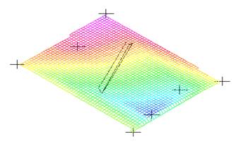
Grid of original topography

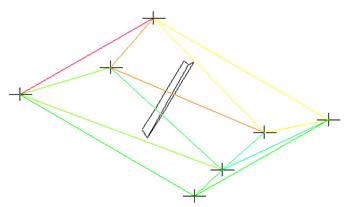
TIN of original seven points

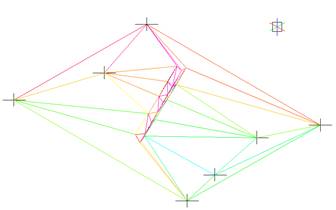
TIN after ditch break line extraction

Subsequently using the TGRD command produces the accurate reproduction as the triangulated grid. The TGRD surface is a TIN which honors both the grid nodes and break lines exactly.

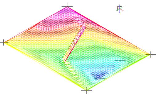
A TGRD gives the best representation

Grids should not be used with surfaces containing break lines. A grid will average across break line and tend to smooth across the breaks. The figure below shows a grid for this same data set.

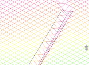
Gridding does not honor break line exactly

Breaks may be established by any MicroSurvey CAD drawing entity, but 2D/3D polylines and 3D Lines are most efficient. Remember that the break line must follow the elevation of the surface to produce meaningful results.

There are two special considerations in break line modeling: vertical discontinuities and intersecting breaks.

Vertical discontinuities

Recall that the MicroSurvey CAD definition of a surface is a single-valued function of the independent variables X, Y. This means that no part of a surface may be exactly vertical, since it would have more than one elevation value at a given X, Y point.

Therefore if you are trying to represent a vertical surface such a wall, you need to offset the coordinates by a small amount. Example top corner of wall could have coordinates of 100,100,100 and the bottom 100.001, 100.001, 90.

Intersecting break lines

MicroSurvey CAD densifies all break lines and resolves all crossing break lines during break extraction. When MicroSurvey CAD processes a single break line, the elevation of the break line itself furnishes the elevation of all densified surface points along it. This produces a potential ambiguity when two break lines intersect over a common X,Y point, yet differ in elevation. Intersecting break lines are representing the same surface; therefore the elevation must be the same at any break line intersection. MicroSurvey CAD resolves this by setting the elevation of the surface to the mean of the elevation values on the two break lines. This feature resolves small measurement and interpolation errors.

To resolve crossing break lines, MicroSurvey CAD must compare every segment of every break line against every other segment. As the number of break lines increases, the computation time increases dramatically.

Stacked data points (multiple control points at a given X, Y location) along break lines are dropped. MicroSurvey CAD resolves stacked data by arbitrarily deleting points from a stack until there is only one. Break lines made up of multiple polylines joined with common endpoints must be treated as break line intersections, which therefore slow processing.

Contours

Menu: MsModeling | Contour

Command: CONT

Icon:

Contours are 2D polylines that follow paths of constant elevation on the modeled surface. Contouring is the interpolation of a specified Z value on a TIN, TGRD or Grid model. Although contours are produced from a surface model, they are not inherently part of the surface model. Contours are always generated on the fly from the surface model of the users choice (Configuration Settings -> Contour).

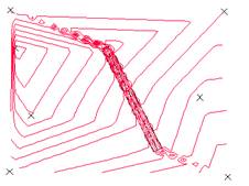
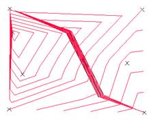
Grid based contours TIN based contours

Contouring from a TIN or TGRD is done via basic linear interpolation which interprets each face of a triangle as a plane in space. Contouring from a Grid is done by linear interpolation on the grid cells. This interpolation is performed by solving polynomial equations representing each triangle of the TIN for a constant Z value. In the illustration above, the same area was contoured on the Grid and the TIN. You can see the TIN edge effects on the TIN based contours.

The segment of a contour line within one triangle or grid cell is always a straight line. Grid cell size therefore has a profound effect on the smoothness or angularity of contours.

Grid Methods

A grid may be calculated by many methods within MicroSurvey CAD. Each of these methods has several options providing for numerous gridding methods.

Continuous Curvature (Standard method)

The Standard method calculates polynomial equations for each individual face of a TIN and evaluates the polynomials at grid vertices that fall under the TIN faces. The user may set the derivatives calculated for each triangle to None, 1st or 2nd in the Configuration Settings -> Grid dialog.

The results are quite different: Using derivatives set to None results in a grid fitted to the TIN in planar fashion. This method involves no polynomial generation. Grid vertices are simply interpolated against the planar TIN faces. Using 2nd derivatives produces a smoothed surface with continuous slope and curvature. This method occasionally may produce surface overshoot problems in areas of very rapid slope changes, but provides excellent results on most data sets.

These continuous curvature methods are the fastest available and provide excellent results when large data sets are to be modeled.

Trend surfaces

The Trend method of gridding allows you to select a particular order polynomial surface and fit it to the entire data set using a least squares fit. You may choose the highest cumulative order of the polynomial in all directions, or specify the order in X and Y directions independently to yield a polynomial with more terms. The selection of a Type 1, first order trend will result only in a least squares fit of a planar surface to the data set. This can be very useful when generating uniformly sloping surfaces to subsequently drape entities onto. Trend surface and trend surface residual generation are also available as surface operations.

Kriging

Kriging is a geostatistical approach to surface generation. Kriging allows the user to design and apply specialized functions to predict the variance the Z value of a surface as a function of distance between control points. The use of kriging requires understanding of semi-variograms and their relationship to spatial distribution of data. When applied without a working knowledge of this theory it is liable to produce inaccurate or deceptive results.

MicroSurvey CAD includes interactive semi-variogram design using the Vario command and supports linear, piecewise, spherical, gaussian and hole semi-variograms. The kriging tools of MicroSurvey CAD are supplied for users already familiar with kriging techniques. This manual does not cover theory related to kriging. Kriging is useful in such disciplines as geophysics, environmental studies, and remediation projects. Users with small contaminant data sets should consider using kriging rather than the standard continuous curvature method.

Grids generated by any of these methods may be used for in any surface operation or for volumetrics, isopachs, profiles, elevation analysis, slope analysis, rendering, or contouring. MicroSurvey CAD can draw grids as 3D face, polyface, 3D mesh, or point entities colored according to the surface colors options.

Chapter 2: Configuring Modeling

Configuration file options

MicroSurvey CAD configuration files are ASCII text files with the extension .QCF. Configuration files are read automatically when MicroSurvey CAD is loaded or you open a drawing. When you open a drawing with MicroSurvey CAD loaded, configuration files will be searched for in the following order:

1. <drawingname>.QCF

2. QS.QCF

If a configuration file with the same name as the drawing exists it is loaded; if not, QS.QCF is loaded if found; if neither is found, MicroSurvey CAD uses its internal default settings. The entire path described by the MicroSurvey CAD path variable is searched.

Saving a configuration file with the same name as the current drawing will cause the configuration to be automatically reloaded the next time the drawing is opened. The entire MicroSurvey CAD environment will be restored automatically.

You may create a standard custom configuration by saving your desired settings to QS.QCF in the directory in which MicroSurvey CAD is installed. After doing so, any drawing without a custom configuration file will use the settings in the QS.QCF file.

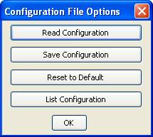
Read Configuration

Menu: MsModeling | Configuration File Options

Reads option settings from a previously saved configuration file, and makes them active for the current surface and drawing. Enter a file name without the .QCF extension or press enter to accept the default of <drawingname.qcf>. When a drawing is loaded with the MicroSurvey CAD Open command, the system will automatically attempt to load options from the default file. If <drawingname.qcf> is not present MicroSurvey CAD will look for a QS.QCF file in along the ACAD search path. If that is not found, MicroSurvey CAD will use its internal defaults.

Save Configuration

Menu: MsModeling | Configuration File Options

Saves the current configuration settings to a named file. Enter a file name without an extension.

Factory Configuration

Menu: MsModeling | Configuration File Options

Resets MicroSurvey CAD Modeling configurations to its internal defaults.

Configuration Settings

Menu: MsModeling | Configuration Settings

Icon:

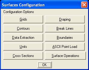
Most of the Configuration settings for the MicroSurvey CAD modeling routines can be made from the Configuration settings dialog as show below.

In this Chapter we will only discuss the most commonly used settings.

Grids Button

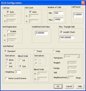
Cell Size

Controls the X and Y dimensions of an individual grid cell. Specify the horizontal and vertical cell size (in drawing units) by entering values in the edit boxes. Selecting the Auto checkbox sets the cell size to 0.0 which causes automatic cell size computation based on the Cell Count setting described below. Non-square grid cells may adversely affect contouring. If you need to change the grid settings after a surface was generated, you will need to delete the grid portion of the surface (clear the grid) before you can generate a new grid using the new values.

Derivatives

Selecting None produces a grid fitted to the planar faces of the TIN. Selecting 1st provides a grid with continuous slope (continuous first derivatives). First derivatives are calculated for each vertex of the TIN and then used to derive the grid. Selecting 2nd provides a grid with continuous slope and curvature (continuous first and second derivatives) of which the theoretical surface honors all control points.

Selecting 2nd is good for uniformly sampled rolling terrain, but can produce over-shoots with very irregularly sampled data or exponential data, such as concentration data. If an overshoot problem exists in the resulting grid, clear the grid, enable the Honor Local Extrema option and recreate the grid. If the problem persists, either add phantom data points to shape the surface or select the None setting for derivatives and recreate the grid.

The derivative setting affects the following commands: Grid, Contour (if contouring on the grid), Drape, Cross-section, Surface region, Track Z and Surface operations

Contours Button

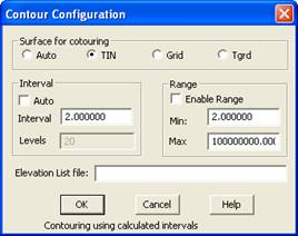
The surface for contouring selection indicates whether you want the contours generated on the TIN, Grid or TGRD. An Auto setting is provided which contours on the grid, unless breaks are present, whereupon it contours on the triangulated grid (TGRD).

Contouring on the TIN builds contours based upon the planar faces of the TIN. Contour lines will be straight lines within any one triangular face of the TIN.

Contouring on the Grid builds contours based upon linear interpolation within each grid cell. Contour lines will be straight lines within any one grid cell. The coarseness or fineness of contours is a function of grid cell size.

Contouring on the TGRD builds contours based upon the planar faces of the triangulated grid. Contour lines will be straight lines within any one triangular face of the TGRD. The coarseness or fineness of contours is a function of grid cell size used when creating the TGRD.

Contour interval

The contour interval is the elevation difference between adjacent contours. You may specify a discrete contour interval, the number of contour interval levels, or choose the automatic setting.

Auto

The Auto check box toggles automatic contour interval calculation. When Auto is selected, the Interval edit box is grayed-out and the Z range of the surface is divided by the number of levels specified below and rounded to an appropriate contour interval.

Interval

Enter the desired contour interval in the edit box. It is possible to set a contour interval which is radically too large or too small. If you do not know the range of your data, choose the Auto check box for the interval and show the contours. Once you determine an appropriate interval, set it in the Interval edit box. The contour interval may also be set directly from the MSModeling pull-down menu (Contour Interval).

Levels

The number of levels is used for automatic contour interval determination. When the Auto button is selected, the Levels edit box becomes available. The Z range of the surface is divided by the number of levels to determine a rough contour interval, and then rounded to an appropriate contour interval.

Range

The range option allows you to only display contours within a specified Z range. This affects both show and draw modes.

Enable range

The enable range check box toggles whether a Z range is used when displaying contours. When Enable range is checked, only those contours within the specified range are displayed. When Enable range is not checked, all contours are displayed.

Min

All contours greater than or equal to the value in the Min edit box and less than or equal to the value in the Max edit box are displayed.

Max

All contours greater than or equal to the value in the Min edit box and less than or equal to the value in the Max edit box are displayed.

Elevation list file

You may enter a file name of an ASCII file containing specific Z values, one per line. If a filename is specified, only contours with those Z values within the file are generated. For example, consider an elevation file containing the following:

Logarithmic contours using an elevation file.

.01

.10

100

1000

Using this elevation file would cause only the six logarithmic contours specified to be drawn.

You may use elevation files to control both the Z value and color of contours generated. If the first line of the elevation file has the word “Color”, followed by a list of (Z value, color number) pairs, then for each Z listed, its contour will be drawn in the corresponding color.

Example color elevation list file:

10,1

20,2

30,3

40,4

An elevation file like this would result in the 10 contour being drawn in MicroSurvey CAD color # 1 (red), the 20 contour in color # 2 (yellow), the 30 contour in green, and the 40 contour in cyan. Using color elevation files, you may totally customize you contouring colors and which contours you wish to display with no alterations to the surface itself.

Data Extraction Button

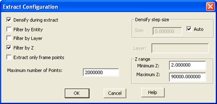
Configure Extract dialog box allows you to filter which entities you extract; densify lines and polylines during extraction; determine whether spline or frame points are extracted from polylines which have been smoothed; and limit the maximum number of points extracted.

Densify during extract

Entities such as 3D lines, 2D polylines and 3D polylines may be densified during extraction. Selecting Densify during extract uses the Densify step size to incrementally step down the entity and create new surface points in addition to the entity’s vertices. This is especially useful when additional points may be needed to adequately describe the surface.

For example, when creating a new topographic surface by extracting digitized contours (2D Polylines), it is common to encounter "flat spots" in some of the drainages in the resulting surface model. These result from not enough control points defining the bottom of the drainage. These may be eliminated by setting OSNAP to ENDPOINT and snapping a 3D polyline down the drainage from one contour to the next. By extracting the newly drawn 3D polyline with Merge Extract with Densify during extract enabled, additional points defining the bottom of the drainage will be added to the surface model. The surface model will now accurately reflect the topography.

Densify step size

If Densify during extract is enabled the Densify step size is used as the increment to step down the entity being densified. In general, you should specify a step length for densification, rather than relying on the Auto setting. The Auto setting chooses a step size based upon the extents of the model, which may not be appropriate for many cases.

Filter by Entity

Enabling Filter by Entity will invoke the entity filter dialog box each time an extract command is used. This dialog will enable you to filter the selected objects by entity type prior to extracting them.

Entity filter dialog box

The Entity Filter dialog lists all of the entity types available and lets you highlight, then select or delete entity types from the list.

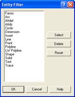
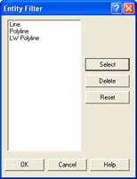
Entity filter dialog before and after selection

Only those entity types remaining on the resulting list will be extracted. A Select button includes entities, a Delete button excludes entities and a Reset button restore the original complete entity list. Press OK when finished.

Filter by Layer

Enabling Filter by Layer allows you to extract only entities on the layer specified in the Layer edit box. This filter may be used together with the other filters. To selectively extract entities from more than one layer, you may repeatedly use Merge Extract and Filter by Layer, specifying different layers each time.

Layer edit box

Enter the layer name to be used with Filter by Layer.

Filter by Z

Enabling Filter by Z allows you to extract only points and vertices with Z values in the range specified in the Minimum Z and Maximum Z edit boxes. Points and vertices with Z values greater than or equal to the minimum Z and less than or equal to the maximum Z will be extracted. By default, MicroSurvey CAD sets the minimum Z to a value of 2. This helps prevent you from extracting insertion points of text and blocks, when extracting data to a surface. If you use the filter options carefully, then you can go below 2 and be safe in not selecting text or block insertion points.

Extract only frame points

Select the check box to extract splined polylines at their frame points only, or leave it blank to extract all vertices.

Maximum number of points

Set the maximum number of points allowed to be extracted to the <.> surface. The default is 2,000,000 points.

Units Button

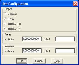
Slope units

Slopes may be specified in degrees, ratio, or in percent. Ratio slope refers to horizontal to vertical ratio (such as 2:1). Percent slope may either be specified as percent slope where 100% slope equals 100 or in decimal percent where a 100% slope equals 1.0.

Area units

Areas by default are returned in square drawing units. You may supply a units conversion factor in the Multiplier box and a text label in the Label box. This will result in all areas being multiplied by the Multiplier and being followed by the area label, such as 1284.2 sq. ft. or 24.3 acres.

Volume units

Volumes by default are returned in cubic drawing units, being

(X units * Y units * Z units). You may supply a units conversion factor in the Multiplier box and a text label in the Label box. This will result in all volumes being multiplied by the Multiplier and being followed by the volume label, such as 32845.3 cu. yds. or 95230.7 barrels.

1 Cubic Foot = 0.037037 Cubic Yards

1 Cubic Metre = 1.307950 Cubic Yards

Boundaries Button

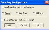
The Configure Boundary dialog controls the criteria for determining when a TIN, TGRD or Grid face is within a boundary.

Boundary method

When a grid or TIN is built with a boundary in effect a grid cell or triangle face may overlap the boundary. You may configure which of the following three methods to use for honoring boundaries.

Center

If the center of the face is within the boundary, draw the face.

Any point

If any vertex of the face is within the boundary, draw the face.

All points

If all of the vertices of the face are within the boundary, draw the face.

There are examples of these settings in Chapter 5: Boundaries.

Chapter 3: Boundaries and Contours

You may limit the area in which Points, Breaks, TINs, TGRDs, Grids, Contours or draped objects are displayed by specifying one or more closed polylines as boundaries with the Set Boundary command. The boundaries may be nested. Boundaries are very useful for presentation purposes.

Boundary Commands

Menu: MsModeling | Boundary Options | Set Boundary

Command: Bound

Icon:

Set Boundary defines an arbitrary boundary defining the area within which MicroSurvey CAD will display a surface. Boundaries affect both draw and show operations. Using boundaries only affects the display of a surface; the surface itself is not modified by the presence of boundaries. The following boundary-smart commands will honor any boundaries in effect:

Points

Breaks

TIN

Grid

Triangulated Grid (TGRD)

Contour

Drape

Post from memory

Surface region

NOTE: Boundaries limit the display of modeling objects to within the boundary. If you forget and leave a boundary set in one area of your model, then move to a different area, you may not be able to display contours, etc. If you attempt to display parts of a surface and don’t see anything, it may be due to having set a boundary which does not overlap the surface.

Establishing boundaries

Boundaries may be extracted from closed 2D or 3D polylines in the drawing or read from ASCII boundary files. Boundaries may be read from and written to disk files with the Read ASCII Boundaries and Write ASCII Boundaries commands as described in the Command reference chapter.

Once a boundary has been selected, it is independent of the drawing entity used to create it. The parent polyline may be erased or frozen with no effect on the boundary.

Prior to running the Set boundary command, the boundary must exist as one or more drawn MicroSurvey CAD entities. They should be either 3D or 2D closed polylines. Although the Set boundary command will close polylines which are not closed, the result may not be identical to the closed polyline if arc segments are involved. Try to always use closed polylines as boundaries. Once a boundary has been selected it stays in effect for the remainder of the drawing session (even if you switch between drawings, until you exit the program), even if the polyline it was created from is erased. Boundaries may be temporarily disabled or permanently deleted with the Set boundary command.

A circle selected as a boundary is ignored completely if drawn as a circle entity and not a polyline; a closed circular polyline arc will be accepted as a circular boundary.

Nested boundaries

You may selectively include and exclude regions by drawing nested closed polylines representing boundaries. The surface will be shown or drawn in any area that is enclosed by an odd number of boundaries, and not in any area enclosed by an even number of boundaries. In the figure below, there is also a boundary around the entire site.

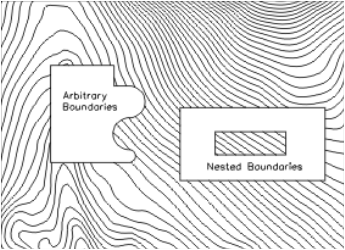
Nested Boundaries

Nested boundaries are used extensively in site planning. Nested boundaries also may be used to prevent dense contours from overlapping map annotations.

Boundaries and surface displays

When a grid or TIN is displayed with a boundary in effect, a grid cell or triangle face may overlap the boundary. The Configuration Settings -> boundary dialog provides for three options to determine whether or not to show or draw a grid cell or TIN triangle. These options are center, any point or all points.

The center option displays the grid cell or triangle if the center of the element is within the boundary. The any point option displays the grid cell or triangle if any vertex of the element is within the boundary. The all points option displays the grid cell or triangle if all vertices of the element is within the boundary.

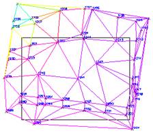
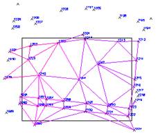
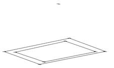
TIN with no boundary TIN with Centre set for boundary honor Set

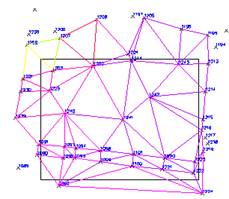
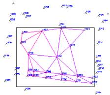
TIN with Any Points Boundary Honor Set TIN with All Points Boundary Honor Set

Note that grid cells and triangles are either displayed completely or not at all; they are not clipped at the boundary. If you want the TIN to follow the boundary exactly, extract the boundary 3D polyline as both a break line and a boundary. This will force the triangulation to follow the boundary exactly, resulting in no triangles crossing the boundary. The Surface region command does this automatically

Contours

Menu: MsModeling | Contour

Command: CONT

Icon:

Contour Interval

Menu: MsModeling | Contour Interval

Command: cont_Interval

Icon:

To change the contour interval uses any of the options shown above. Note if there are existing contours in the drawing you will have to redraw the contours at the new interval to see any changes. (draw the contours on a different layer or erase the originals)

Contour Configuration

Menu: MsModeling | Configuration Settings | Contours

Command: QSCONFIG

Icon:

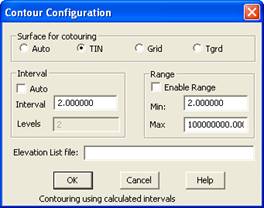
SEE PREVIOUS SECTION FOR DETAILED INFORMATION ON THE ABOVE TOGGLES.

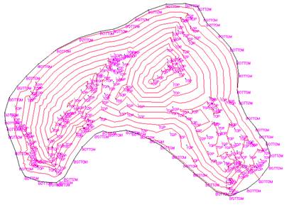
Contours based on a normal TIN without derivatives

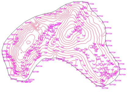
Contours based on a Grid.

Contour Labeling

Menu: MsModelling menu | Annotate | Label Contours

Command: _LABEL

Contour labels can be added to the contours, no matter how they were generated.

There are two methods to label contours;

1) is to manually select each location, 1 at a time,

2) is to draw a control polyline that the labeling routine will follow and label each time it crosses a contour.

1) When you run the routine the first prompt you will see is:

Enter text height <2.000000>:

Enter a valid text height in units, or pick two locations on screen to measure between and use that value.

Next you will choose between trimming the contour line or using a wipeout to hide the contour line. Trimming the contour actually breaks it into 2 pieces whereas the wipeout option simply hides the contour.

Trim/Wipeout <Trim>:w

Now you can start picking locations on the contour lines to label, one at a time.

Select label location (Undo/Control): <pick>

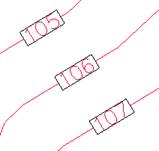
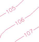
If the wipeout frame is on you will see boxes around the labels (seen above).

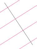
To remove this box run the Wipeout command and turn the Frames OFF (seen below).

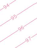
2) To use the Control Polyline method, you need to actually draw the polyline prior to starting the labeling command. The polyline should cross each contour only once.

When you run the Contour Labeling command, follow the prompts as seen above but when you are asked

Select label location (Undo/Control):c <type in C>

NOTE: Contours that cross the control line twice may only be labeled once.

Draw your control line so it only crosses a contour once.

After the above note is presented, you will be asked to select the contours to be labeled. You can use any selection method to accomplish this.

Select contours to label:

After you have selected all of the contours to be labeled, press enter and then pick the control polyline.

Select Polyline Control line:

The contours will be labeled and the polyline will be erased, leaving you with a nice clean set of labeled contours.

Chapter 4: Drape and Flatten

Drape

Menu: MsModeling | Design Tools | Drape

Command: Drape

Icon:

Drape is a very powerful tool. Any object may be translated vertically until its Z values conform to the current surface. Drape creates a new draped 3D drawing entity and deletes the original source entity.

Drape may be used to solve for the Z value of a surface at a group of points such as construction stake-out plans, fluid flow or finite difference model nodes. It is particularly useful for combining 2D maps and 3D models of the same area, by converting 2D map data into 3D data draped on topography. Any line or polyline draped onto the surface becomes a 3D profile. Exploded hatch patterns may be draped on a surface to create 3D thematic maps.

Concepts

Drape alters drawing entities so they conform in elevation to the current surface in surface memory. Draping a point entity is the simplest case. The Z value of the point entity is changed such that it lies in the surface. How this elevation value is solved for is determined by the Configure Drape settings.

Drape Configuration

Within the Configuration Settings -> Drape dialog you may specify to drape to the Planar TIN, TIN (using curvature), TGRD or Grid.

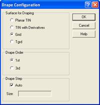
Draping requires a surface to contain a TIN, TGRD or Grid. You can not drape to a surface containing just points.

The Planar TIN represents the surface as the TIN with no curvature within any one triangular face. The elevation of a point or node is calculated on the planar triangular face. If a linear entity (line or polyline) is draped using this method, vertices are only added where it crosses a triangle edge. This results in the least number of vertices in the draped line, yet it honors the surface exactly.

Draping to the TIN uses the derivatives along with the TIN to drape on the complete mathematical description of the surface, including breaks if present. This is more accurate than draping on the TGRD or Grid, which represent a sampling of the mathematical surface at an interval based on the cell size used. Because derivative (slope and curvature) information is used, the settings for Derivatives in the Configure Grid dialog are used. Specifying None is the same as Planar TIN above. Specifying 1st or 2nd uses continuous slope or continuous curvature respectively.

Draping to the TGRD or Grid interpolates between the triangle or grid cell vertices, rather than solving the underlying mathematical surface. Draping to the TGRD or Grid does make sense in cases where the grid or TGRD nodes have been modified with surface operations such as Max, Min, or Trend, which alter the node elevations without respect to the TIN and derivatives.

Drape step

When draping an object consisting of lines and arcs, each segment is subdivided based upon drape step size into smaller segments by adding vertices. Each of these densified vertices is then draped onto the surface and becomes a vertex of a new 3D polyline resulting from the Drape command. The Configure Drape dialog controls drape step size. Drape step is ignored when draping to the Planar TIN.

Draping off the edge of a surface

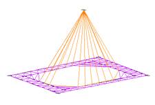
If an entity, such as a line or polyline, extends past the edge of the defined surface, those parts of the line which do not overlie the defined surface are set to a constant elevation referred to as drape base. The elevation used for drape base is set in the Undefined grid value edit box within the Configuration Settings -> Grid dialog. It is a good practice to only drape entities which entirely overlie the surface or to use a boundary to clip them during draping if needed.

Drape and Boundaries

If a boundary is enabled using the Set Boundary command, Drape only creates objects within the defined boundary. For example, if a rectangular boundary is in effect and a line to be draped extends outside of the boundary, the resulting 3D draped polyline will only be created within the boundary. No entities will be created outside of the boundary. As a consequence of this, draping an entity which lies totally outside of a boundary will not produce any resulting entity. This will have the same effect as an erase, because Drape erases the source entity and in this case produces no new entity.

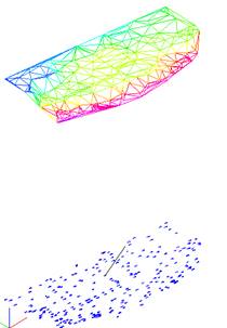
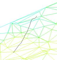
2D line before being draped Line after being draped on the surface

Flatten

Menu: MsModeling | Design Tools | Flatten

Command: MSFlatten

Icon:

Flatten creates a 2D elevation profile of a 3D polyline. Typically the 3D polyline being flattened has been draped so it lies within the surface.

The Flatten command prompts for 3D polyline(s) to flatten and then asks questions regarding graph scaling and labeling. The first vertex of the 3D polyline selected becomes the left end of the profile. Flatten and Cross-section expect polylines drawn left to right. Use the Swappoly command to reverse any 3D polylines which are drawn in the wrong direction prior to using Flatten.

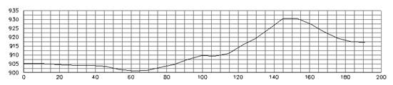
Profile created using the flatten command on the line draped in the previous section.

When the command is executed you are prompted to:

1. Select Entities: Pick the object(s) that you would like to present on the profile grid.

2. You will then be prompted for the Vertical multiplier at the command line. The default is 1 which means the vertical scale will be the same as the Drawing Scale. If you use a vertical multiplier of 5 and your drawing scale is set to 1”=50’, then the vertical scale will be 1”=10’.

3. You will then be prompted for the vertical and horizontal spacing and labeling interval. Enter the desired number or accept the defaults by pressing Enter.

4. You will be prompted to pick the location in the drawing where you would like the profiles inserted. The origin point is at the lower left corner of the graph.

The Profile label text will use the current size available in the drawing (last size used).

Chapter 5: Surface Operations

Surface operations allow you to perform mathematical calculations between surfaces. Surfaces may be copied, renamed, deleted, and read from or written to disk. Individual parts of one or more surfaces may be selectively cleared. Surface operations allows inspection of detailed surface statistics for any surface.

Menu: MsModeling | Surface Operations

Command: DSOP

Icon:

Surface operations dialog box

Surface management and surface algebra are accomplished by invoking the surface operations dialog box from the menu.

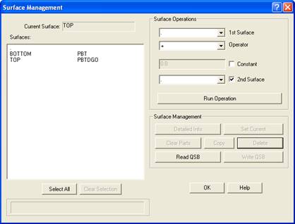
Surface Operations dialog

The surface operations dialog has three main divisions. The surface list is in the upper left quadrant, the mathematical controls are in the upper right quadrant with the surface management buttons beneath them.

Surface list

The surface list displays the names and component parts of the currently defined surfaces. The name of the current surface is displayed above the surface list. The operation of the surface list is the same as the Layer Control dialog box in MicroSurvey CAD. Surfaces in the list may be selected or deselected by picking them with the mouse. When a surface is picked, it is highlighted. Pressing any of the enabled surface management buttons along the bottom of the dialog box will operate on the highlighted surfaces.

For example, selecting one surface and pressing the Current button makes that surface the current surface. Selecting several surfaces and pressing the Delete button deletes the selected surfaces from surface memory.

Each line of the surface list contains the surface name and a list of the component parts which currently exist. Some examples:

. P T

Existing P TDG

Proposed PBTD .PBT

The surface name is followed by letters corresponding to existing parts. The letters represent the following parts:

P Points

B Breaks

T TIN

D Derivatives

G Grid

Parts listed after the period (such as the .PBT in the Proposed surface) represent parts of the triangulated grid (TGRD).

In the list above, the results surface <.> contains points and a TIN. The Existing surface contains points, TIN, derivatives and grid. The Proposed surface contains points, breaks, TIN, derivatives, as well as points, breaks and TIN in the TGRD.

Surface management buttons

The surface management buttons operate on the highlighted surfaces in the surface list. The buttons may be grayed-out if unavailable for the selected surface(s). For example, if more than one surface is selected, the Current button is unavailable because you may only have one current surface.

Select All

Highlights all surfaces in the surface list.

Clear All

Clears the highlighted selections in the surface list. This is simply de-selecting any highlighted surfaces in the list. This command does not affect the contents of any surface.

Current

Sets the current surface. The current surface is offered as the default surface name for any command involving a surface. The Current button is only available when one surface is selected from the surface list.

Read QSB

Invokes the standard file dialog box to read a MicroSurvey CAD binary QSB file which has been previously saved.

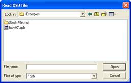
QSB files are created by the Write QSB command or the Load ASCII Table command (QSML). All of the surfaces in the QSB file are loaded into surface memory. Any existing surface in memory with the same name as a surface in the file is overwritten without comment or warning. If you wish to load only selected surfaces from the file, rather than all surfaces, use the SOP Read command from the keyboard, which will prompt you surface by surface for which surfaces to load.

Write QSB

Writes selected surfaces to a binary QSB disk file.

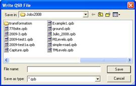
The highlighted surfaces will be written. Write QSB invokes the standard file dialog box to write a MicroSurvey CAD binary QSB file. The QSB file has a file extension of .QSB. A QSB file is a very efficient way to store surface information. All surface parts and descriptions are stored in the file, but boundary and window information (if any) are not. Reading a QSB file written with this command restores all of the written surfaces to surface memory.

Clear Parts

Invokes the Clear Parts dialog box, allowing you to remove any or all parts from the selected surfaces.

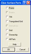
The Clear Parts dialog lists all of the parts of the selected surface(s) and allows you to pick which ones are to be removed. In this way specific parts, such as the TIN, Grid or TGRD, may be removed from a surface.

Copy

Copies the contents of a selected surface into another surface. With the surface to be copied selected, press Copy and a small dialog pops up allowing you to enter the new surface name.

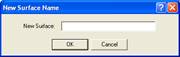
If the new surface does not exist, one will be created under the name supplied. If it does exist, its contents will be replaced by the new contents.

Delete

Deletes the highlighted surfaces from memory. Deleting the results <.> surface will produce an empty <.> surface; deleting a named surface will eliminate it completely. MicroSurvey CAD drawing entities that have been generated with the Draw option will not be affected.

Detailed

Displays the detailed surface information for one surface, including surface description, associated MicroSurvey CAD layer, surface method, and surface statistics including number of points; minimum and maximum of X, Y, Z, and slopes; plan and surface area; and volume. The Detailed button is enabled only when a single surface is highlighted in the surface list.

If more than 10,000 points are in a surface, you will be given a chance to skip area and volume statistics calculation.

There may be a pause when invoking the detailed listing while MicroSurvey CAD calculates the area and volume statistics. The areas and volumes reported will be in square drawing units or cubic drawing units unless a user-specified units have been defined in the Configuration Settings -> Units dialog box.

Pressing the Detailed button invokes the following dialog box.

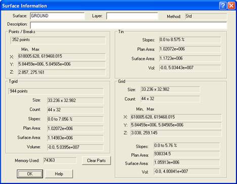
Surface Information dialog

Within the detailed Surface Information dialog, you may change the name of a surface, add a detailed description for the surface, or create a link between a surface in surface memory and a layer in the MicroSurvey CAD drawing. The dialog box show above has all parts shown for purposes of illustration, normally a TGRD and Grid don’t co-exist in the same surface.

Surface, Edit Box

The surface edit box displays the surface name. You may change the name of a surface by altering the name in the edit box.

Description, Edit Box

You may enter a surface description (up to 100 characters) which will be carried for the rest of the drawing session and included in any QSB file you may save. The description field for the results surface is automatically filled by the surface operation which created it with a description of the operation performed.

Layer, Edit Box

Associates a MicroSurvey CAD drawing layer with a MicroSurvey CAD surface. Any MicroSurvey CAD-generated drawing entity related to this surface will be placed on this layer. When you select the Draw option from the Points, Breaks, TIN, TGRD or Grid commands, the entities drawn will be placed on the designated layer.

This operation overrides the current drawing layer as set by the MicroSurvey CAD Layer command. If no layer is specified, MicroSurvey CAD always draws to the current layer or Layer 0 (zero) depending upon the routine..

Surface statistics

Statistical information on each surface part is displayed in the surface information dialog box. Number of points, minimum and maximum values for X, Y, Z, and slopes are displayed. Plan area, surface area and volumes are computed for TIN, Grid and TGRD parts. All computations encompass the entire surface.

Note that the memory used by the surface is displayed at the lower right of the dialog box. Deleting surfaces frees memory and makes it available to MicroSurvey CAD.

Clear Parts

See details above in previous section.

Chapter 6: Volumetrics

Fast, accurate volumes are very important in most surface modeling applications. Within MicroSurvey CAD, volumes may be computed directly from surfaces residing in surface memory using the Surface volume or Area volume command or computed from a drawn TIN, TGRD or Grid using the Volume by entity command. None of these volume functions use the current boundary which may have been set with the Set Boundary command, rather they may prompt for one or more closed polylines representing areas under which to calculate volumes. The closed polylines can be the same polylines used to create your boundaries.

TIN based volumetrics

MicroSurvey CAD calculates volumes of a surface by summing the volume underneath each face of the surface within the area specified. A face may represent either the triangles of a TIN or Triangulated Grid; or the rectangular grid cells of a Grid.

Volume under a triangle

For any surface with a TIN, calculating a volume consists of calculating the volume under each triangle in the desired area and summing the result. Remember that regular TINs and Triangulated Grids are both types of TINs. First let’s look at one triangle of a TIN and determine its volume.

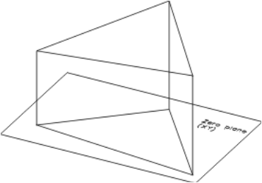
Volume under one triangle

The volume under a triangle is measured relative to the zero (XY) plane. The Z value of the surface used in a volume command represents thickness. If you use the Surface volume or Area volume commands, you may also calculate the volume between two surfaces or the volume between a surface and a constant. In these two cases, MicroSurvey CAD calculates the thickness surface and places it in the results <.> surface. A Z value of zero in this surface represents zero thickness. All volume calculation is then performed on this thickness surface.

If you have subtracted an existing topographic surface from a proposed topographic surface, areas of fill will have positive thickness values and areas of cut will have negative thickness values. When volumes are then calculated, positive (fill) values are calculated as positive volumes and negative (cut) values are calculated as negative volumes. Reversing the order of the surfaces in the calculation will reverse the sign (+/-) of the resulting volumes.

Volume under a surface

Calculating the volume under a surface consisting of triangles is accomplished by summing the individual volumes of the component triangles within the area to be calculated. To accomplish this we would use the Surface Volumes command.

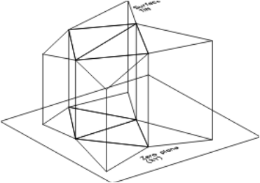
Volume under part of a TIN

Entire surface

If we want the volume under an entire TIN, we may simply draw the TIN and use the Volume by entity command and select the drawn TIN. If the TIN was drawn as a polyface mesh, select the one polyface entity. If the TIN was drawn as individual 3D faces, select all of the 3D faces. It is easier to use the Surface volume command which returns the same result, but does not draw any MicroSurvey CAD drawing entities.

Partial surface volume

To calculate a partial volume on a surface we would use the Area Volume command. It calculates the volume under one or more sub-areas of surface in surface memory. Each sub-area is defined by selecting a closed polyline representing the area under which the volume is to be calculated. You may select as many sub-areas as you wish. This is the primary volumetric tool because there is no ambiguity on the boundaries of the calculated volume. Think of each area polygon as a "cookie-cutter" which is vertically punched through the surface(s). The surface must exist for the entire area that the closed polyline covers.

Volume calculation from surface memory

Volumes may be computed directly from surfaces residing in surface memory using the Surface volume, and Area volume command. None of these volume functions use the current boundary which may have been set with the Set Boundary command, rather they prompt for closed polylines representing areas under which to calculate volumes if areas are required. These two commands both invoke the same dialog box.

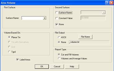
Surface Volume dialog box

Volume calculation options

Volume may be calculated between a surface and the zero plane (i.e. sea-level), between a surface and a constant elevation, or between two surfaces. If the volume requested is between two surfaces or between a surface and a constant, the results surface <.> will contain the actual thickness surface for which the volume is calculated. You may show or draw this surface to confirm its geometry. You could also copy the <.> surface to a new name so you can preserve it as the <.> surface will be over-written again with the next calculation. Always inspect the thickness surface prior to volume calculation by showing the TIN, TGRD or Grid from an oblique viewpoint or by contouring it. In some cases the edges may contain anomalies; either correct the surface or exclude the edge effect by using Area Volumes.

Within the dialog box you may specify the basis for the volume (Planar TIN, TIN with derivatives, Grid or TGRD, depending upon what is available for the surfaces), the first surface, optionally a second surface or constant, and output file name and type.

Basis for volume calculation

Planar TIN Calculate volumes based on the planar TIN.

TIN w/ Deriv Calculate volumes using the TIN and derivatives.

Grid Calculate volumes based on the Grid.

TGRD Calculate volumes based on the TGRD.

The volume will be computed on the selected surface part. If the part does not exist, the selection will be grayed-out. The Planar TIN selection will always be available and a TIN will be created if required.

First surface name

Select the surface under which to calculate volumes from the surface pick list. If this surface represents thickness, the volume should be computed between this surface and the zero (XY) plane. In this case you would specify None for the second surface. If the volume to be computed lies between two surfaces or between one surface and a constant elevation you will need to specify the second surface or constant.

Second surface name

If the desired volume is between two surfaces, click on the check box next to the surface pick list and select the second surface from the pick list. A new surface representing the difference between the two surfaces (first surface minus second surface) is computed and placed in the results <.> surface and the volume is calculated.

Internally this computation uses the TIN, derivatives, grid and/or TGRD with the Maximize option within the surface operation subtract. This insures the most rigorous resulting thickness surface. If you want curvature used when calculating the volume between two surfaces, use the TIN with derivatives option.

Two surface example

If you have two surfaces EXISTING and PROPOSED and select PROPOSED as the first surface and EXISTING as the second surface, the results <.> surface will contain your cut/fill surface. Positive areas (P - E > 0) represent areas of fill and positive volumes represent the fill volumes. Negative areas (P - E < 0) represent areas of cut and "negative" volumes represent the cut volumes. Positive and negative volumes represent the volumes above and below (respectively) the zero (XY) plane of the surface being computed. The net volume reported is the sum of positive and negative volumes. When the net volume equals zero, the cut and fill volumes are the same.

Selecting Surfaces for a Two Surface Volume Computation

The "New minus Old" rule of thumb can be used as a guideline when selecting surfaces for either a volumetrics computation or a surface operation that involves two surfaces. This allows you to resolve ambiguity over the meaning of positive and negative volumes.

Examples of applying the "new minus old" rule:

Comparing an ORIGINAL GROUND Surface against an ASBUILT stockpile surface:

Select ASBUILT (new or present surface) as the 1st surface

Select ORIGINAL GROUND (old or past surface) as the 2nd Surface

· The volume of fill (materal that is added to ORIGINAL GROUND to reach ASBUILT) will be listed as Positive Volume

· The volume of cut (material that is subtracted from ORIGINAL GROUND to reach ASBUILT) will be listed as Negative Volume

Comparing an ORIGINAL GROUND Surface against a TAILINGSPOND surface:

Select TAILINGSPOND (new or present surface) as the 1st surface

Select ORIGINAL GROUND (old or past surface from before excavation) as the 2nd Surface

· The volume of fill (materal that is added to ORIGINAL GROUND to reach TAILINGSPOND) will be listed as Positive Volume. This will likely be the smaller quantity if there is any at all.

· The volume of cut (material that is subtracted from ORIGINAL GROUND to reach TAILINGSPOND) will be listed as Negative Volume. This will likely be the larger quantity.

Comparing an ORIGINAL GROUND Surface against a DESIGN surface:

Select DESIGN (new or future surface) as the 1st Surface

Select ORIGINAL GROUND (old or present surface) as the 2nd surface

· The volume of fill (materal that is added to ORIGINAL GROUND to reach DESIGN) will be listed as Positive Volume

· The volume of cut (material that is subtracted from ORIGINAL GROUND to reach DESIGN) will be listed as Negative Volume

Constant

If the desired volume is between a surface and a plane of constant elevation, select the check box next to the Constant selection and enter the constant value in the edit box. A surface representing the difference between the first surface and the constant (first surface minus constant) is computed and placed in the results <.> surface and the volume is calculated.

This option is convenient for determining reservoir volumes at different water levels.

None

The volume between the first surface and the zero plane is computed. Select the check box next to None. Use this for computing the volume of a surface already representing thickness.

File output

The resulting volumes are always displayed on the text screen, but may be optionally written to a text file. Select the check box of the desired option and press the File button and supply a file name up to eight characters in file dialog. The appropriate file type (.txt) will be appended.

ASCII Writes an ASCII text file.

None Does not write a file.

If a volume units conversion factor and units name has been specified in the Configure Units dialog, the volumes will be converted and displayed in the specified units.

Label areas

Area volume allows for the volumes under multiple sub-areas of the surface to be calculated. When multiple area polygons are selected, selecting the Label Areas checkbox will cause each polygon to be sequentially labeled with area numbers. These area numbers correspond to the area numbering in the volume report. The labels are placed on the current layer, in the current text style, and at a text height equal to the grid cell size, unless overridden by a current text style containing a fixed text height. The areas are numbered in the order the are selected.

Running a volume command

After selecting the options in the Surface or Area Volume dialog box and pressing OK, you are prompted to select area polygons (if Area Volumes is being run) and the calculated volumes are displayed on the text screen. The volume results are written to the file or database table if requested.

Volumes reported

The volume report produced looks similar to the following:

VOLUMES: Reported in Cu.Yds.

Using 0.37037 cubic units/Cu.Yds.

Area Positive Volume Negative Volume Net Volume

1 15025.1 14215.5 809.6

2 10215.3 9812.4 402.9

3 982.5 3402.5 -2420.0

Total 26222.9 27430.4 -1207.5

For each area three numbers are reported:

Positive Volume: The positive volume within the area polygon.

Negative Volume: The negative volume within the area polygon.

Net Volume: The net sum of volumes within the area polygon.

A Total Positive Volume is reported representing the total positive volume of the entire surface. A Total Negative Volume is reported representing the total negative volume for the entire surface. Positive volumes represent areas with Z values greater than zero and negative volumes represent areas with Z values less than zero.

If you have selected a volume conversion factor and unit name in the Configuration Settings -> Units dialog box, the volumes reported will have the conversion factor applied and the units name will be displayed. There is no validity checking on user-supplied units conversion factors.

The three variations of the volume command are individually described below.

Volume by Entity

Menu: MsModeling | Volumetrics | Volume by Entity

Command: Volume

Volume by entity calculates the volume under MicroSurvey CAD drawing entities. Unlike Surface volume and Area volume which operate on surfaces in memory, Volume by entity only operates on drawing entities such as meshes, polyface meshes and 3D faces drawn with the TIN, TGRD or Grid commands.

Volume by entity

Return to select all visible or

Select objects: select

Select objects via the normal MicroSurvey CAD object selection methods. MicroSurvey CAD will calculate the volume under the selected entities in cubic drawing units. 3DFACEs, Polyfaces, and 3D polygon meshes are the only entity types that will yield a volume; all other entities are ignored. The status bar will be updated with the total as it is calculated. Volume by entity computes three results: a positive volume for objects above the zero datum (x,y) plane, a negative volume for objects below the zero datum plane, and a net volume.

Volume by entity always calculates volumes relative to the zero plane (XY plane) of world coordinate system. If you want the volume calculated with reference to a different plane from the zero datum, use the MicroSurvey CAD Move command to move the drawn TIN or GRID vertically to the desired level.

Either grid cells or triangles may be used to compute a volume under a surface, but they generally yield slightly different results: triangles are treated as flat faces, whereas the grid represents uniform sampling of a smoothed curved surface that passes through all the control points. If the grid is a 3D polygon mesh, a single value of volume for the entire mesh is calculated. If the grid consists of individual 3DFACEs or Polyfaces they are calculated for all selected faces, then summed and reported.

If the resultant faces extend both above and below the zero datum, those faces above the zero plane are reported as positive volumes and those faces below the zero plane are reported as negative volumes. If a single face penetrates through the zero plane, a single net volume is calculated for that face, rather than separate positive and negative portions.

All of MicroSurvey CAD’s volume commands will produce identical results when run on the same surface parts. Volumes run on a TIN, TGRD and Grid of the same surface will yield different results, because of different amounts of curvature information carried by the different surface parts. TGRDs and Grids may reflect surface curvature, regular TINs do not. Always visually examine a surface prior to calculating its volume.

Surface volume

Menu: MsModeling | Volumetrics | Surface Volumes

Command: SVOL

The Surface volume command calculates the volume under an entire surface in surface memory. If you are using this volume to compare to a volume computed under a different surface, you must insure that the areas covered by the two surfaces are identical. They should use the same points on the perimeter or surface juts may give incorrect answers in areas where no valid data can justify the surface.

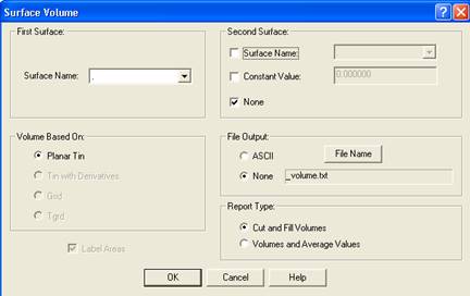
Surface Volume dialog box

Area Volume

Menu: MsModeling | Volumetrics |

Command: AVOL

The Area volume command calculates the volume under one or more sub-areas of surface in surface memory. Each sub-area is defined by selecting a closed polyline representing the area under which the volume is to be calculated. You may select as many sub-areas as you wish.

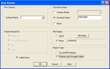
Area Volume dialog box

Caution: Area polygons should not overlap!

Be careful not to overlap or nest area polygons, or incorrect results will be obtained. If your area polygons are adjacent to one another use OSNAP when constructing the polylines to insure that adjacent area polygons share vertices.

The surface part used for volume calculation (TIN, Grid or TGRD) must be defined in the area covered by the area polygon. If a surface is not defined under part of an area polygon, the undefined area contributes no volume to the reported volumes.

Volumes may be calculated between a surface and the zero plane (i.e. sea-level), between a surface and a constant elevation, or between two surfaces. If the volume requested is between two surfaces or between a surface and a constant, the results surface <.> will contain the actual surface for which the volume is calculated. You may show or draw this surface to confirm its geometry.

Internally, Area Volume performs the same sequence as described in the Surface volume example earlier in this chapter. Each area polygon is conceptually draped on the surface, densified and used as a break as well as a boundary, then the volume is computed within the area polygons boundary. This is done for all area polygons selected and the report is written to a file or database file.

Volume calculations

When calculating a volume, you must choose whether to base the volume on the TIN, the Triangulated Grid or a regular Grid. The choice depends upon whether break lines are present in your surface and whether surface curvature between data points is desired. The differences are listed below.

Planar TIN Planar faces, honors breaks, no curvature

TIN w/ deriv. TIN (using curvature for drape), honors breaks

Grid No break lines, uses curvature if present

TGRD Break lines and curvature

Planar TIN volumes

Calculating the volume from a TIN uses the planar faces of the triangles for volume calculation. Break lines are honored exactly by the TIN. TINs are used for data sets in which there is sufficient control that inter-point curvature may be ignored or is not desired. Examples include volumes on sites with dense control (such as dense contours or points from a stereo-plotter) or sites with mainly break lines such as benched pits.

Choosing TIN based volumes means that linear interpolation between the points and densified break lines accurately describes the surface.

TIN volumes using derivatives

Calculating the volume from a TIN with derivatives uses the planar faces of the triangles of the <.> surface for the actual volume calculation, but uses curvature (derivatives) internally when draping one surface to the other to determine thickness. Break lines are honored exactly by the TIN. TIN with derivatives is used for volumes between two surfaces in which inter-point curvature is significant. Examples include volumes on sites with sparse control on one surface where MicroSurvey CAD-supplied curvature is needed to properly represent the surface.

Grid volumes

If your surface contains break lines use the TIN or TGRD for volumes.

Calculating the volume from a Grid uses the average elevation for each grid cell multiplied by its plan-view area for volume calculation. Grids are used for data sets which have no break lines and inter-point surface curvature is desired. Examples include volumes on sites with sparse control (such as spot elevations on rolling topography) or sites with smooth rolling surfaces and no break lines.

Choosing Grid based volumes means that a grid accurately describes the surface, even though the grid will not have grid nodes exactly at control points. If you choose Grid based volumes on a surface containing break lines, an error message will result. Surfaces containing break lines should have volumes based on either the TIN or TGRD, because a grid tends to average across break lines.

TGRD volumes

Calculating volumes using TIN with derivatives is usually more efficient.

Calculating the volume from a TGRD (Triangulated Grid) uses the planar faces of the triangles of the TGRD for volume calculation. Break lines are honored exactly by the TGRD. TGRDs are used for data sets in which both inter-point curvature and break lines are needed. Examples include volumes on sites with rolling topography mixed with abrupt cuts, ditches or walls. A golf course green together with its associated sand traps would be such a case: Curvature is needed on the green and in the bottom of the sand traps, but the edge between the sand traps and the green will be break lines. The TGRD is a special type of TIN which has densified vertices along break lines and vertices at grid nodes away from the break lines which honor surface curvature. The resulting surface honors both curvature and break lines.

Choosing TGRD based volumes means that both breaks and surface curvature are needed to accurately describe the surface.

Boundary conditions

The surface must be defined everywhere underlying the area polygon for which volumes are to be calculated. If the area polygon extends past the defined surface, only the part of the surface within the polygon will be calculated. Any portion of the area polygon without the surface underlying it is assigned a volume of zero.

It is a good practice to display the TIN, Grid or TGRD (using the Show option) in plan view and compare them to your area polygons prior to calculating a volume. This allows you to confirm that the surface is defined everywhere beneath your area polygons. If your area polygon extends past the edge of your surface, you have two choices: Alter the area polygon or extend the surface by adding additional control points.

Remember that Area volume does not allow nested or overlapping polygons. Nested polygon cases may be accomplished using boundaries, draped polylines as breaks and the Volume by entity command.

If you are using Volume by entity, you must drape the area polygon onto the surface, then extract it as both a break and a boundary, prior to drawing the TIN. In this case it is extremely important that the draped polyline (now a 3D polyline) reflects the correct Z value as it traces the area boundary. Always inspect the TIN visually prior to calculating volumes.

Comparison to Average End Area volumes

Some users may be familiar with Average End Area volume calculation, rather than TIN based calculation. Average End Area calculations involve generating a series of sections across the model, then multiplying the average area of adjacent sections by the distance between them and by the total number of sections. The implicit assumption is that the change in the surface between adjacent sections is linear and no surface curvature occurs between sections. To approximate this, many sections must be created. Yet in the end, the problem with Average End Area is the first word in its name: Average. The accuracy of the result is variable, depending upon section spacing. An infinite number of sections would be required in order to calculate an accurate result.

The TIN honors every data point exactly and the volume beneath each triangle of the TIN is a discrete fixed volume, not an average. A TIN based model is faster, more accurate, and simpler to use.

Common volume calculation mistakes

The most common user mistakes in calculating volumes relate to boundary conditions. The following guidelines should be reviewed:

· If the difference between two surfaces is used, both original surfaces must be defined under the area to be calculated.

· Area polygons should not overlap or be nested.

· Inspect the surface visually by contouring it in plan view or viewing the TIN, Grid or TGRD from a perspective view prior to calculating the volume. Is it reasonable?

· Calculate the volume of the appropriate surface part based on the guidelines in Practical volume calculations earlier in this chapter.

· If you are comparing resulting volumes calculated from different surfaces, they must be computed under exactly the same area to have any meaning.

· If you are using a volume conversion factor in the Configure Units dialog box, a mistake in entering the conversion factor will be reflected in all volumes reported.

Chapter 7: Exercises:

Calculating the Volume of a Stock Pile.

1. For this exercise we will use the job called Stock Pile.dwg.

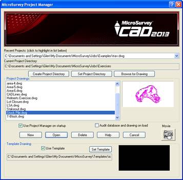
Pick on the drawing name and then pick Open,

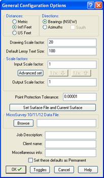
Pick on OK to continue past the MicroSurvey General Configurations Options dialog to see the following drawing on screen.

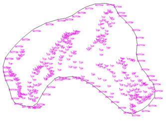
What you have here is a stock pile of material which was surveyed. The points around the base of the pile have all been labeled as BOTTOM and all internal shots were labeled as TOP. A 2D Polyline, drawn at zero elevation, connects all of the BOTTOM points, like a cookie cutter.

What we need to do is create 2 surfaces, 1 for the bottom shots only and 1 for the top of the pile matching back to the bottom points. This way we can accurately calculate the volume of this pile, between the two surfaces. The polyline will be used to ensure we do not include any surface information outside of the pile, which could introduce some error.

2. To start with we should check a few settings to make sure they are as we require. Go to the MsModeling menu | Configuration Settings.

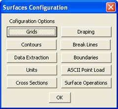
In this dialog, pick on the Units button.

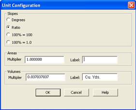
To display Volumes in Cubic Yards rather than Cubic Feet, we need to enter the correct multiplier and suitable Label.

Pick OK to return to the previous dialog, and OK again to exit the command.

3. Now we will generate the two surfaces. We will do this in two different ways, just so you can see them both. First we want to create the top surface from the drawing.

Go to the MsModeling menu | Extract from Drawing | Extract to Surface.

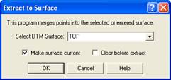
We will name this surface as TOP. Pick OK to continue.

The top surface will actually contain all points in this pile, both points labeled as TOP and BOTTOM. So on the command prompt you can either window the entire job or simply press enter to select the entire job. You should see the report:

340 points total in surface.

4. We can now create a TIN of this surface, so we can examine the surface to ensure it is correct and there are no anomalies.

You can type in the command TIN or go to the MsModeling menu | TIN Create/Edit | .

On the command line you will see the following prompts:

: tin

current surface <TOP>:(or Select) ß <enter>

None/Show/Draw/Redraw <Show>?d ß D for Draw <enter>

Lines/Faces/Polyface <Polyface>: ß <enter>

Select Invisiblity...All/Interior/None ß <enter>

653 triangles built

Creating boundary set...

Creating polyface points, Please Wait...

Creating faces...

You will see the TIN.

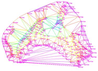
What do you notice immediately? There are extra triangles across open void areas where no stock pile material exists. This is why we have the polyline tracing the bottom points. This will let us ignore these external triangles when we do an Area Volume.

Now we need to look at the surface in 3D to check for any other issues. Go to the View menu | Real-Time motion | Real-Time Sphere.

Using your mouse, pick and hold the left button and as you move your mouse you will rotate the drawing in 3D.

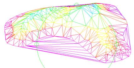
Now you can spin the drawing around to ensure the TIN looks valid. If you were to find an issue, you would need to go back to your original data and correct the problem, re-extract the point data to the surface and redo the TIN again. In this example, our data is just fine.

5. You can exit the command by pressing ESC or press Enter. To return to aplan view type in the command PLAN and press ENTER TWICE in a row. Now we can delete the TIN. We can delete the TIN from the drawing because the surface remains in memory, so it can still be used for volume calculations later.

6. Now we will create the BOTTOM surface. To do so go to the MsPoints menu | Active Coordinate Editor.

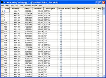
This brings up a list of all of the coordinates in this job. We will sort them based upon Description by double clicking on the header DESCRIPTION.

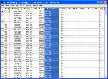
Take your mouse and pick and drag starting at point 1 all the way down to the last point with the descriptions BOTTOM (point 381).

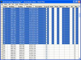
Once those points have been all highlighted, either right click on the highlighted area, or go to the Edit menu. Pick on Add Selection to DTM Surface.

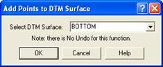
Name the surface BOTTOM and pick OK to continue.

You will go back to the Active Coordinate Editor – you can exit it as well.

On the command line you will see:

Points extracted from 58 entities.

58 points total in surface.

58 points added to surface.

7. We can now create a TIN of this surface, so we can examine the surface to ensure it is correct and there are no anomalies.

You can type in the command TIN or go to the MsModeling menu | TIN Create/Edit | .

On the command line you will see the following prompts:

: tin

current surface <.>: (or Select)S ßS to bring up the dialog to select from

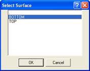Pick on BOTTOM and pick OK.

None/Show/Draw/Redraw <Show>? D ß D <enter>

Lines/Faces/Polyface <Polyface>: <enter>

Select Invisiblity...All/Interior/None<enter>

89 triangles built

Creating boundary set...

Creating polyface points, Please Wait...

Creating faces...

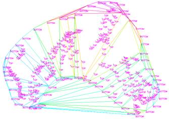
The first thing you should notice is the same external triangles as the TOP surface had.

We could look at the tin in 3D but it would simply reveal a flat surface as expected.

8. To do a volume between these two surfaces and not have any possibility that the external triangles could give any errors, we need to drape the polyline onto both surfaces and extract the draped polyline as a breakline for each respective surface. This ensures that all triangles inside the pile hit the edge of the pile in the same way so all edge triangles cover the same area along the edge.

In this case, the perimeter of the pile is the same for both the TOP and BOTTOM surfaces (being they both used the same points to form the perimeter), so the polyline can be draped to either surface and then extracted as a breakline to both surfaces.

To clean up the screen, erase the tin off the screen (remember it stays in memory).

Go to the MsModeling menu | Design Tools |

On the command line you will see:

: drape

current surface <BOTTOM>:(or Select) <enter>

Return to select all visible or

Select entities: ß pick the polyline <enter>

Entities in set: 1

Select entities: <enter>

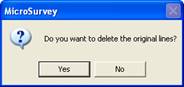
Answer YES to delete the original Polyline.

9. Now we need to extract this polyline to each of the two surfaces, as a breakline.

Go to the MsModeling menu | Extract from Drawing |

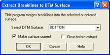
Pick OK to continue, as we will do the BOTTOM First.

On the command line you will see something like this:

Return to select all visible or

Select entities: ß Pick the draped polyline <enter>

Entities in set: 1

Select entities: <enter>

Using a curve error of 0.117432

1 Break Lines extracted

Auto densification...

418 triangles built

456 triangles built

190 additional points added to current surface

Run the command a second time – this time select the TOP surface.

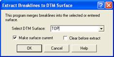
On the command line you will see something like this:

Return to select all visible or

Select entities: ß Pick the draped polyline <enter>

Entities in set: 1

Select entities: <enter>

Using a curve error of 0.117432

1 Break Lines extracted

Auto densification...

982 triangles built

1048 triangles built

204 additional points added to current surface

Now we have two surfaces that have triangles that have the same edges around the perimeter. So now we can do an Area Volume Calculation.

10. Go to the MsModeling menu | Volumetrics |

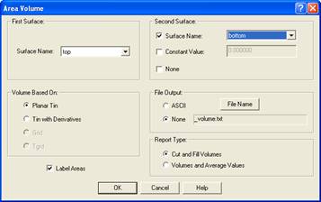
Enter in the first surface name (TOP) and the Second Surface name (BOTTOM). There are two different reports that can be generated, we will examine the Cut and Fill Volumes first.

Pick OK to continue, then pick the polyline around the stock pile, to calculate the volume within.

VOLUMES:

Reported in Cu. Yds.Using 0.037037037 cubic units/Cu. Yds.

Volume of TOP-BOTTOM based on a planar tin.

Area Positive Volume Negative Volume Net Volume

---- --------------- --------------- ----------

1 2130.812 -1.062e-014 2130.812

So the answer in this example is 2130.812 cubic yards.

To generate the Volumes and Average Values report, rerun the command and select that option.

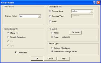
VOLUMES:

Volumes reported in Cu. Yds.Using 0.037037037 cubic units/Cu. Yds.

Volume of TOP-BOTTOM based on a planar tin.

Area Net Volume Plan Area Average Z

---- ---------- --------- ---------

1 2130.812 8082.228 7.118

This report not only gives you the Net Volume but it also reports the plan area within the polyline and average depth of material over the site, if you were to level the pile.

If you want volumes of sub-portions of the pile, you could draw another polyline around the sub-portion, drape it to the two surfaces as appropriate, then extract the draped polylines as breaklines. Then do an area volume between the two surfaces within the selected polyline.

Simple Road Exercise

Because of the size and complexity of this tutorial we have broken it down into 11 smaller steps to make it easier for you to follow.

Step 1) Opening the Job

Step 2) Create the Ground Surface

Step 3) Rendering the Surface

Step 4) Inputting the Horizontal Alignment

Step 5) Stationing and Saving the Horizontal Alignment

Step 6) Create Profile

Step 7) Design New Profile

Step 8) Create Cross Section Template

Step 9) Create New Road Surface

Step 10) Output Cross Sections

Step 11) Saving the Drawing and Surfaces

Step 1 - Opening the Job

Start by opening the CONTOURS.DWG file from the Project Manager. The CONTOURS.DWG file should reside in your C:\Documents and Settings\UserName\My Documents\MicroSurvey\MSCAD\2013\Jobs2013\Examples directory by default. (where UserName is the user logged into that computer)

Pick on the job name and then pick the Open button.

The system General Configuration Options should be set to match the following for this job to work cleanly. Press the OK button once they are confirmed to be correctly set.

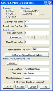
You will see a series of contours and a few points. They will be used to define your existing surface.

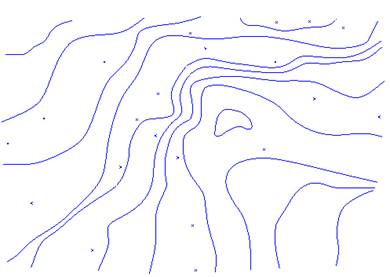
Do the SAVEAS command to create a new drawing using the contours as a starting point. This will protect the original data so you can execute the exercise again if you wish.

Type SAVEAS and press enter, or go to the File pulldown menu and pick on the SAVEAS command.

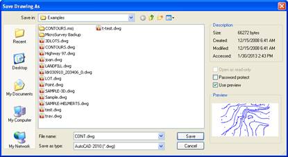
Change the default folder to save in C:\Documents and Settings\UserName\My Documents\MicroSurvey\MSCAD\2013\Jobs2013 (where UserName is the user logged into that computer) and change the file name to CONT.DWG then pick the SAVE button to continue.

Step 2 - Create the Ground Surface

Next, we need to extract all of the 3D point data and 3D breaklines (contours) to create the existing surface.

To set the program up so we can select only the data required to extract to a surface, we need to go to the MsModeling menu | Configuration Settings.

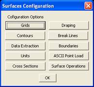
Pick on the Data Extraction button

Turn on the toggle for Filter by Entity and set your Density Step Size to 2 by turning the Auto option off.

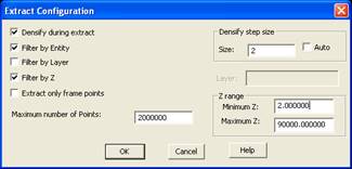
Pick OK to return to the previous dialog and OK again to exit the dialog.

Next we will load the Modeling toolbar by right clicking on any existing toolbar on screen (see toolbar menu on right). The following toolbar will appear on screen. Move it to a convenient location on your screen (can be docked anywhere you wish).

To extract points to a surface, pick this button.

The following dialog box will appear. Please fill it out as shown below and then pick the OK button to continue.

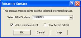
After picking the OK button you will be asked to Pick the correct items from a filter list, to extract entities from the drawing. You will then see the following dialog:

Pick on POINT and then pick the Select button.

Points will now be the only entity that can be selected.

Pick OK to continue:

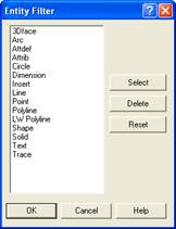
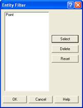
The command line will now display:

Return to select all visible or

Select entities:

We need all of the points on screen to form the top surface so simply press the ENTER button to grab them all.

It should report in the command prompt area;

21 points total in surface.

So far we have the points that help define the surface but we now also need the breaklines.

To extract the breaklines to the same surface, pick this button.

The following dialog box will appear. Please fill it out as shown below and then pick the OK button to continue.

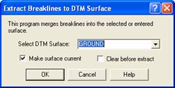
After picking the OK button the Entity Filter dialog will come up again.

It will default to only points being the list. Pick Reset to see the complete list. Then pick on LW Polyline and the select button to short list it to only the LW Polyline.

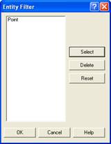
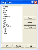
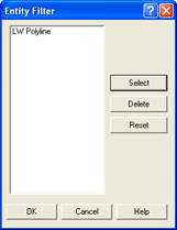
Pick OK to continue:

The command line will now display:

Return to select all visible or

Select entities:

We need all of the linework on screen to help form the top surface so simply press the ENTER button to grab them all.

The command line will now display:

1916 additional points added to current surface

Next we need to create a TIN for this surface. Pick this button. from the palette.

The TIN command will ask you several questions. Answer them as follows;

current surface <GROUND>:(or Select): <Enter>

None/Show/Draw/Redraw <Show>? <Enter>

This will temporarily display the TIN on screen, so we can confirm that the TIN has been generated correctly.

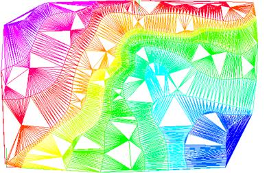
A redraw or zoom command will remove the TIN from the screen. The Tin will remain in memory.

Step 3 – Exploring the Surface in 3D

To look at the surface from any 3D angle, we would first need to Draw the surface to our screen, rather than just using the Show option.

To control what layer the TIN is drawn on, go to the MsModeling menu | Surface Operations (or pick on this toolbar button ) to bring up this dialog.

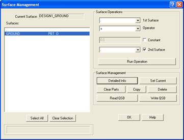
Highlight the Ground surface and then pick the Detailed Info button to bring up the next dialog.

At the top in the middle of this dialog, you can control what layer the TIN will be drawn on.

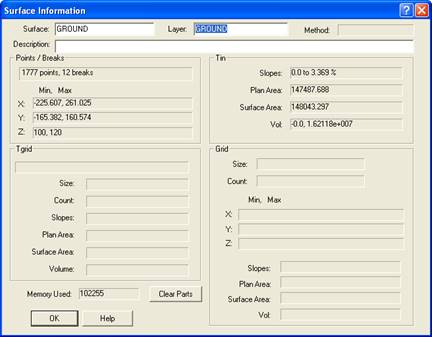
Set it to GROUND and pick OK to return to the previous dialog. Then pick OK again to exit the dialog.

Now we can draw the TIN into our drawing. Pick this button. from the toolbar.

The TIN command will ask you several questions. Answer them as follows;

Surface name <GROUND>: <Enter>

None/Show/Draw/Redraw <Show>? D <Enter>

Lines/3dFaces/Polyface <Polyface>: <Enter>

Select Invisiblity... All/Interior/Between breaks/None <None>: <Enter>

Now the TIN will be part of the drawing and drawn on layer Ground.

To make it easier to view, we will isolate the ground layer, so nothing else is on screen.

You can do this by going to the MsTools menu | Layer Control |

Select entities: ß pick the TIN you just drew

Entities in set: 1 <enter>

Select entities: <enter>

Now all you have on screen is the TIN layer.

Go to the View menu | Real-time Motion | Real-time Sphere and use the left mouse button to pick and hold while you move the mouse, to see the surface rotate in 3D.

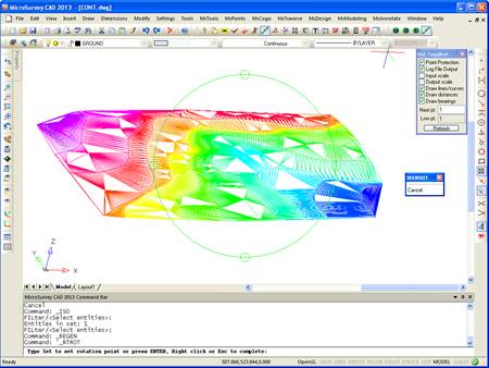
You can spin the surface around in real time by use of the mouse.

You can now exit the command by pressing enter or ESC. You can return to plan view by typing PLAN and pressing ENTER TWICE in a row.

To bring the rest of the layers back to the screen go to the MsTools menu | Layer Control | .

The TIN does not need to remain in the drawing for the rest of the exercise, and can be deleted by going to the Edit menu | Delete, and picking the tin to select it, and press enter to complete the command.

Step 4 - Inputting the Horizontal Alignment

Now that we have our surface we can create our alignment.

Start by going to the MsDesign pulldown menu | AutoRoute and picking the command.

In the Command prompt area, it will ask you the following, please enter the information shown:

Enter name for horizontal alignment: <>: MAPLE

* NOTE *

When naming a horizontal alignment, be sure to use only a single word, with no spaces, as the name, such as:

ROAD1, Orange_Side_Road, Maple_Street, Pine-Street, Maple

From point: -200,100

To point: 1,90

To point: 70,-45

To point: 240,-50

To point: <Enter>

Note: It is not necessary to enter exact coordinates to create an alignment. You can also "pick" the points on screen using Object Snaps, as appropriate.

The center line of the road is now drawn.

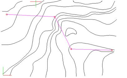
Next you will be asked if you wish to edit the alignment:

Answer Yes so we can insert new curves and spirals.

Edit alignment. Add/Delete/Move/sHift/Curve/Scs/Tangent: SCS

Select POT (or linework) to add/edit scs: <pick the red circle at the FIRST bend in the road> (zoom in if you can not pick it easily. Don’t miss it!)

Now you will see the following dialog box.

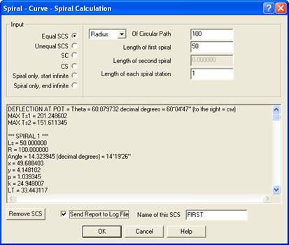
Fill in the values shown on the dialog above, and the calculations are automatically updated.You can name the spiral-curve-spiral and export the report to the View Log file.

Pick the OK button to place the spirals and curve on the screen.

Select POT (or linework) to add/edit scs: <Enter>

Edit alignment. Add/Delete/Move/sHift/Curve/Scs/Tangent: Curve

Select POT (or linework) to add/edit curve: <pick the red circle at the SECOND bend in the road> (zoom in if you can not pick it easily. Don’t miss it!)

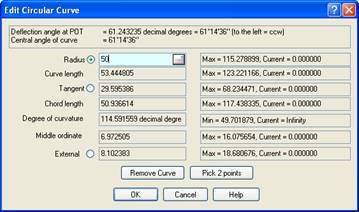
Enter curve radius: 50

The rest of the curve data it automatically calculated and displayed in the dialog.

Pick OK to draw the curve to the screen.

Select POT (or linework) to add/edit curve:<Enter>

Edit alignment. Add/Delete/Move/sHift/Curve/Scs/Tangent: <Enter>

Now you will be asked if you wish to continue and profile the existing ground surface?

Pick NO for now.

At this point your job should look like this (your colors may be different):

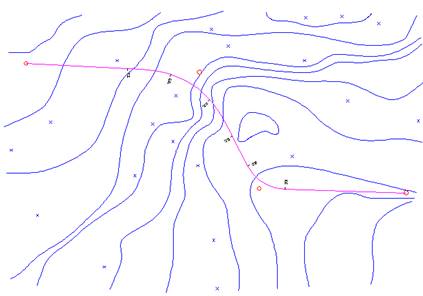
Step 5 - Stationing and Saving the Horizontal Alignment

Before we continue with the profile lets label the stationing along the alignment.

Go to the MsDesign pulldown menu | AutoRoute pick on the Label Alignment option

Label alignment. Stations/Offsets/Newpt/Existingpts/Report: S

STATIONS

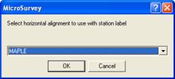
There are many options to label and create points along the alignment and on offsets, as well as reports.

We are going to simply label points along the centerline in this example.

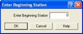
Pick OK to continue

After picking the Alignment name and beginning station, you will have the following dialog box appear:

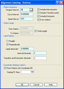
Fill in the table as shown and pick OK to continue.

Label alignment. Stations/Offsets/Newpt/Existingpts/Report:ENTER

Here is what you will see on screen,

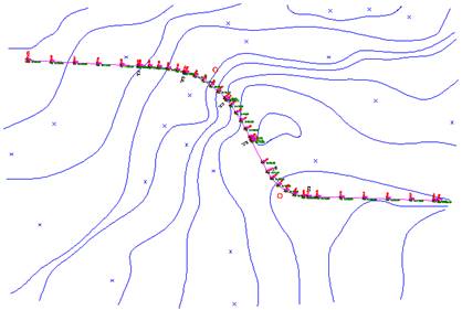
and a close up showing a portion of the labeling,

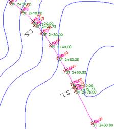
You can see that the tangent, curve and spiral have had the stationing labeled, as well as the beginning of Curve and Spiral. New points have been created along the centerline with the description set as the station. Some text overlap is apparent and a simple move command can clean this up.

Now we should save this alignment to a file to protect us and allow us to retrieve it without having to recreate it from scratch.

Under the MsDesign pulldown menu | AutoRoute pick on the Write .HRZ File option.

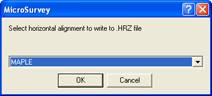confirm the alignment name and pick OK to continue.

On the command prompt window you will see the message that tells you where and what the file is called.

Alignment saved in C:\Documents and Settings\Glen\My Documents\MicroSurvey\MSCAD\2013\Jobs2013\MAPLE.HRZ.

Here is the contents of this file:

HRZVERSION=3::MAPLE

100.00000000,-200.00000000,0.00000000

90.00000000,1.00000000,0.00000000,50.00000000,50.00000000,1.00000000,1,100.00000000,0

-45.00000000,70.00000000,50.00000000,0,0,0,0,0,0

-50.00000000,240.00000000,0,0,0,0,0,0,0

Step 6 - Create Profile

Now that we are finished labeling and saving the horizontal alignment – lets continue with the vertical profile.

Go to the MsDesign pulldown menu | AutoRoute and pick the Extract Existing Ground Profile option.

You will be asked to pick from a list of surfaces – we want GROUND as our surface.

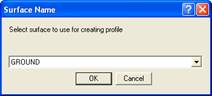
Pick on the word GROUND and pick the OK button.

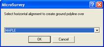
Confirm the alignment you are working with and pick OK to continue.

Next you will be shown a dialog box that will control how the profile will be drawn.

Change the settings to match this dialog:

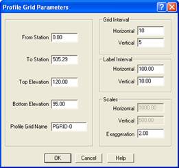
The only value you need to change is the Grid Interval Horizontal from 100 to 10. Press the OK button to continue.

Pick lower starting corner of grid: <Pick Somewhere Appropriate – maybe Above the Alignment>

You will be asked if you wish to create the design profile?

Answer NO for now.

Now let’s set the Profile_Grid layer to gray (color 9) for easier visibility, Go to the Explore Layer button and pick on it.

Then pick on the layer name above, and change the color to gray(9).

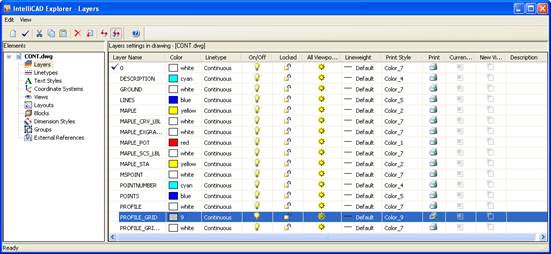
The close the dialog to continue.

Now the profile will look like this:

Step 7 - Design New Profile

Now that we have had a chance to look over our existing profile, we now need to create a design alignment.

Go to the MsDesign pulldown menu | AutoRoute and pick on the Design Vertical Alignment option.

Draw new profile grid or use existing New/<Existing>: <Enter>

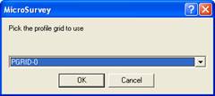
Confirm the grid to work on and pick OK to continue:

Enter name for vertical alignment: <>: MAPLE

NOTE

When naming a Vertical alignment, be sure to use only a single word, with no spaces, as the name, such as: ROAD1, Orange_Side_Road, Maple_Street, Pine-Street, Maple

At this point, the program will draw a rubber band line from the bottom left corner of the graph. This helps you to find the starting end of the profile. Pick on the graph where you wish to start the new profile line.

Pick first VPI location: < pick near the left edge around the existing profile>

Change the dialog box that comes up, so the station and elevation look like the following;

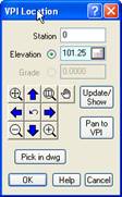
Pick the OK button.

Next pick somewhere around the middle of the profile and change the dialog box so the station and elevation match the following;

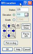
Pick the OK button.

and lastly pick over near the top right and change the settings so the station and elevation match the following.

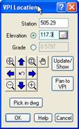
Pick the OK button.

Press ENTER to continue.

Next you will be asked:

Pick YES to continue.

Now you will be prompted,

Add/Curve/Delete/Move/Freezethawgrid:CURVE

Select VPI (or linework) to add/edit curve: <Pick the Red Circle at the FIRST bend in the vertical alignment> (zoom in if you need to, to be able to pick the red circle cleanly – don’t miss it)

Current curve length (in stations) = 0.000000

Select method to define curve length: Pick/Type: TYPE

Enter curve distance: 150 <Enter>

Select VPI (or linework) to add/edit curve: <ENTER>

Add/Curve/Delete/Move/Freezethawgrid: <ENTER>

Next you will be asked if you wish to pass our cross section template along the design alignment and create a new surface.

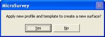
Answer NO for now because we need to create the template first.

Before we create the Cross Section Template, lets label the vertical curve.

Go to the MsDesign pulldown menu | AutoRoute and pick on the Query/Label VPI option.

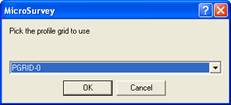
Confirm the vertical alignment grid to use, pick OK to conitue:

Select existing VPI: <Pick the Red Circle at the FIRST bend in the vertical alignment> (zoom in if you need to, to be able to pick the red circle cleanly – don’t miss it)

You will see the following dialog box.

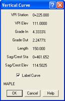
Be sure to pick the Label Curve box to turn it on. Then pick the OK button to continue.

The curve will be label as shown below:

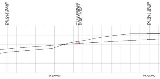
Select existing VPI:<enter>

Now to give us a copy of the vertical profile in a file,

Go to the MsDesign pulldown menu | AutoRoute and pick on the Write .VRT File option.

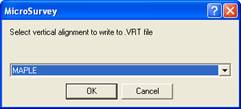
Confirm the vertical alignment and pick OK to continue.

The command prompt will display the following to confirm it was saved.

C:\Documents and Settings\Glen\My Documents\MicroSurvey\MSCAD\2013\Jobs2013\PGRID-0.VRT saved.

Here is the contents of this file:

VPI 1 STA 0.000 Z 101.250

VPI STA 225.000 Z 111.000 L 150.000

VPI STA 505.290 Z 117.300 L 0.000

END

Step 8 - Create Cross Section Template

Now you will create a template for our road cross section.

Go to the MsDesign pulldown menu | AutoRoute and pick on the Create Cross Section Template option.

You will see a template editor on screen. This editor has many options that can be filled out.

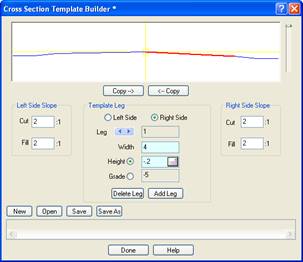
We will use the default settings.

Switch to Leg 2 on the right and set the width to 1 and height to -0.8

Switch to Leg 3 on the right and set the width to 1 and height to 0

Then pick the ßCopy button to mirror the section.

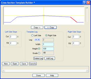
Pick the SAVE button. This will allow you to save the template for future use in this and any other project.

Give the template the name of MAPLE, as shown.

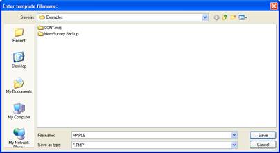
Pick the SAVE button to continue.

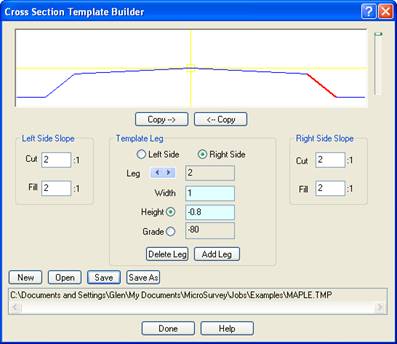
The file name and location will now be displayed in the dialog.

Pick DONE to continue.

The following message is also placed in the command prompt window.

Cross section template file saved as C:\Documents and Settings\Glen\My Documents\MicroSurvey\MSCAD\2013\Jobs2013\MAPLE.TMP.

Step 9 - Create New Road Surface

Now that the cross section template is complete, we can now apply it to the design alignment.

It is important that the entity filters that may have been used when creating the original surface are disabled before continuing this operation. Go to MsDesign | Msmodeling |

Configuration Settings | Data Extraction

In the dialog shown, uncheck “Filter by Entity”

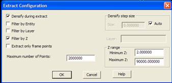
Go to the MsDesign pulldown menu | AutoRoute and pick on the Create New Design Surface option.

You will then see the following dialog box:

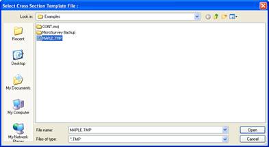
Pick on our MAPLE template then pick the OPEN button to continue.

The following dialog comes up next,

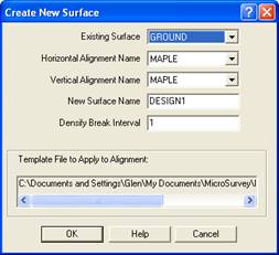
You need to confirm the surface and alignment names match the box shown above. Press the OK button.

After a short period of time (a few seconds or so), the following prompt appears in the command window.

Draw or Show new TIN? Draw/Noshow/<Show>:

Press enter to default to Show

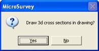
Answer YES

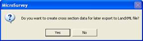
Answer YES

This will export a LandXML file that will be able to be uploaded to our FieldGenius data collector, for use in the field, or to many other programs that can read this file format.

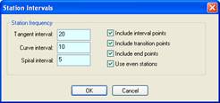
Set the intervals as show. Pick OK to continue.

Your drawing should now look something like this:

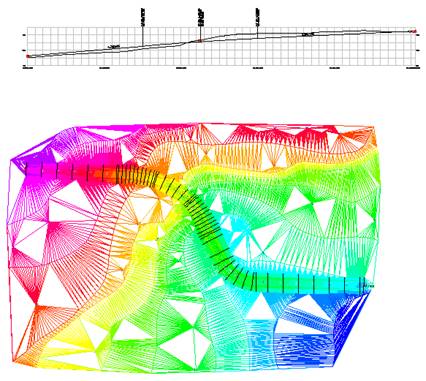
After seeing the TIN you can hit the redraw button to clear the TIN. The Surface does stay in memory for future use.

What you will now see on screen is the road with the template applied, showing the outer edge where the template intersects with the original surface.

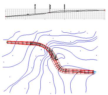
Step 10 - Output Cross Sections

Now lets get some cross sections along the alignment.

Go to the MsDesign pulldown menu | AutoRoute and pick on the Extract Cross Sections from Alignment option.

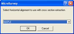
Confirm the Alignment and pick OK to continue.

Be sure to set the next dialog box exactly as shown below to ensure you get the correct results. Special attention to ensure you select BOTH surfaces as shown.

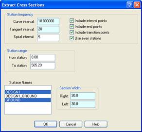
Pick the OK button to continue.

Answer YES.

This will draw lines on the plan view of the alignment to show where the cross sections will be extracted from.

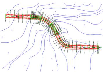
Then:

Answer YES then you will have only the 3D section lines left.

When you answer YES you will be shown another dialog box that controls the output of the sections. Please fill it out exactly as shown:

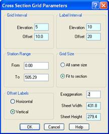
Pick the OK button to continue.

Pick lower left corner: <this is the starting location for the sections to be drawn> (go to the right of the drawing so they do not overlap on screen)

You will see the sheet size outlined and the sections draw within the sheet.

Changed the color of Layer GRID to gray (9) as we did for the profile, above. Here is a close up of a few of the sections:

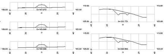
Step 11 – Saving the Drawing and Surfaces

Be sure to save the drawing and the surfaces.

To Save the Drawing, Simply pick on the Save button or go to the File menu and pick on the Save command. Your finished drawing should look something like this:

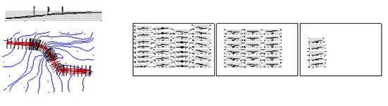
To save the surfaces you need to go to the MsModeling menu | and this dialog will come up:

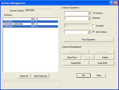
Pick on the 2 surfaces as shown above and pick the Write QSB button.

Enter in the file name CONT and pick Save.

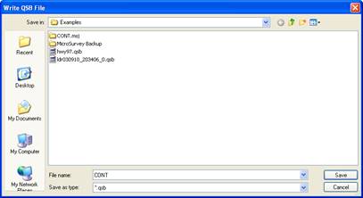
Pick OK to exit the command.

Now the surfaces and the drawing are both safe! You can now exit the program with the ability to reopen the drawing and reload the surface file, if you need to do further work in it.

Adding Sewers to our Road Design

We need to insert a base structure to start with. Go to the MsDesign menu | Sewer/Storm Mains | Layout Sewer Network.

On the command line you will be asked the following:

Insert new or connect to existing structure. Connect/Insert/Join <Insert>:

Press enter and you get the following dialog:

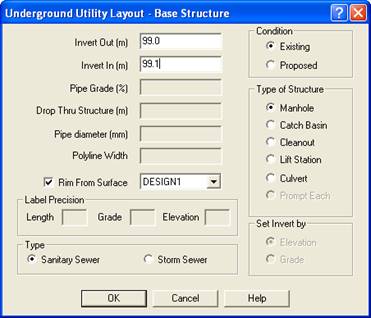
From here you decide if this is going to be an Existing sewer line or a Proposed sewer line, Sanitary or Storm. You can also tell it what type of structure is to be placed. The inverts and if the Rim is from the surface, and which surface to use.

Once you set all of this you pick the OK button to be able to place the structure and a number for the structure.

Pick structure location: -173,87 ß coordinate we will use

Enter structure number <1>: ß Structure number

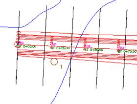
Now that we have the first structure placed, we need to add the remaining structures to the network.

Go back to the MsDesign menu | Sewer/Storm Mains | Layout Sewer Network

Insert new or connect to existing structure. Connect/Insert/Join <Insert>: C

Type in C to connect to a structure – then pick the previous structure we inserted.

You will then be asked:

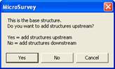
Pick YES so we will be adding our network so this is the base structure.

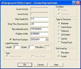
Enter the data as show and pick OK to place the next structure.

Pick next structure location: 5,79 ß coordinate we will use

1 structures found.

Enter structure number <2>: ß Structure number

We will continue to add 2 more structures in this network

Pick next structure location: 85,-32 ß coordinate we will use

2 structures found.

Enter structure number <3>: ß Structure number

Pick next structure location: 230,-39 ß coordinate we will use

3 structures found.

Enter structure number <4>: ß Structure number

Pick next structure location: Press enter to be prompted to select a structure

Select a structure: Press enter to exit command

Above is a snapshot of the last 2 structures. Notice the labeling between the structures along the pipe.

MsDesign menu | Sewer/Storm Mains | Station/Offset/Rim

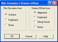
We will use the Surface for the RIM elevation and stationing from the alignment.

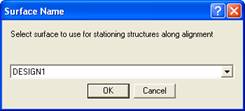
Confirm the surface to work with.

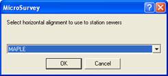
Confirm the alignment to work with.

Select first structure (downstream): ß Structure #1

Select last structure (upstream from previous selection): ß Structure #4

NUM = 1: STATION = 0+027.613, OFFSET = 11.642, RIM = 101.462

NUM = 2: STATION = 0+203.791, OFFSET = -10.048, RIM = 109.488

NUM = 3: STATION = 0+345.368, OFFSET = -10.484, RIM = 114.993

NUM = 4: STATION = 0+494.973, OFFSET = -10.701, RIM = 115.814

The station and offset of each structure is displayed, in relation to the alignment and the rim elevation is displayed based upon the surface.

MsDesign menu | Sewer/Storm Mains | Tag Manholes

You pick on each of the manholes, one at a time, and place the tag information. Here are examples of the 4 structures being tagged.

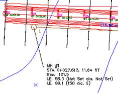
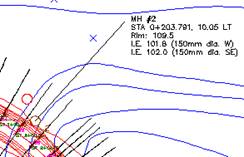
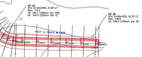
MsDesign menu | Sewer/Storm Mains | Table of Structures

Select structures to include in table:

Select entities: all ß either pick them all or type in all

Entities in set: 4

Select entities:

4 structures found.

Pick location for upper left corner of table: ß Pick off to the side somewhere

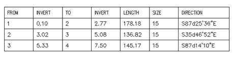
Here is what my diagram looks like so far:

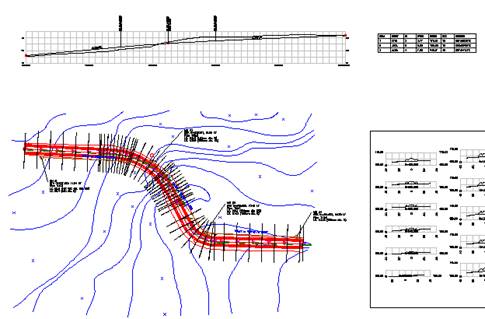
MsDesign menu | Sewer/Storm Mains | Auto Profile

Select first structure (downstream):

Select last structure (upstream from previous selection):

Draw new profile grid or use existing New/<Existing>: ß press enter for existing profile

(This will be the same profile used for the road.

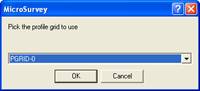
Pick OK to continue:

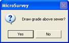
Pick NO.

Your sewer profile is drawn on top of the road profile:

Here is a blowup of the first portion:

INDEX

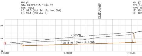
Area Units................................................................ I

Area volume command............................................ I

Average End Area volume....................................... I

Boundaries............................................................... I

Boundaries and surface displays.............................. I

Boundary conditions................................................ I

Boundary method..................................................... I

Boundary smart commands..................................... I

Breakline Definition................................................ I

Breaklines................................................................ I

Breaks...................................................................... I

Brealines.................................................................. I

Cell Size................................................................... I

Clearing parts........................................................... I

Colors....................................................................... I

Commands............................................................... I

Common volume calculation mistakes.................... I

Comparison to Average End Area volumes............ I

Configuration files................................................... I

Read Configuration.................................................. I

Save Configuration.................................................. I

Constraining to a Z range........................................ I

Continuous Curvature (Standard method)............... I

Contour colors......................................................... I

Contour Configuration............................................. I

Contour Interval....................................................... I

Contour labels.......................................................... I

Contour Settings...................................................... I

Contouring specific elevations only;Logarithmic contours I

Contours................................................................... I

Definition;Grid;TGRD............................................ I

Elevation list file...................................................... I

Contours................................................................... I

Copying.................................................................... I

Cross Section Template........................................... I

Cross Sections.......................................................... I

Setting the current surface....................................... I

Derivatives concepts;slope calculation.................... I

Setting Derivatives;Slope control............................ I

Factory Configuration;Configuration, resetting defaults I

Definition................................................................. I

Delauney criterion................................................... I

Deleting.................................................................... I

Densify during extract............................................. I

Densify step size...................................................... I

Description field...................................................... I

Detailed listing......................................................... I

Dialog box............................................................... I

Display problems..................................................... I

Drape........................................................................ I

Drape and Boundaries.............................................. I

Drape step................................................................ I

Draw versus Show................................................... I

Enable range............................................................ I

Establishing boundaries........................................... I

Exploring a Surface................................................. I

Extract dialog box.................................................... I

Extract Existing Ground Profile.............................. I

File output................................................................ I

Filter by Entity......................................................... I

Filter by Layer......................................................... I

Filter by Z................................................................ I

Flatten...................................................................... I

Derivatives setting................................................... I

Grid.......................................................................... I

Parts of;Points;TIN;TGRD...................................... I

Grid.......................................................................... I

Grid methods........................................................... I

Trend surfaces.......................................................... I

Kriging..................................................................... I

Grid volumes........................................................... I

Honor Local Extrema.............................................. I

HRZ file................................................................... I

Intersecting Breaklines............................................ I

Kriging..................................................................... I

Layer........................................................................ I

Layer Isolate............................................................ I

Layer UnIsolate....................................................... I

Surface memory....................................................... I

Logarithmic contours............................................... I

Modeling Surfaces................................................... I

MSFlatten................................................................ I

Nested boundaries.................................................... I

Orbit Command....................................................... I

Partial surface volume............................................. I

Parts of a Surface..................................................... I

Planar TIN volumes................................................. I

Points....................................................................... I

Points, Definition..................................................... I

Practical volume calculations.................................. I

About....................................................................... I

QSB files.................................................................. I

QSX.......................................................................... I

Read QSB................................................................ I

Reading.................................................................... I

Real-Time Sphere.................................................... I

Renaming................................................................. I

Results <.> surface.................................................. I

Road Design Tutorial............................................... I

Step1.................................................................... I

Step10.................................................................. I

Step11.................................................................. I

Step2.................................................................... I

Step3.................................................................... I

Step4.................................................................... I

Step5.................................................................... I

Step6.................................................................... I

Step7.................................................................... I

Step8.................................................................... I

Step9.................................................................... I

Saving...................................................................... I

Saving Surfaces....................................................... I

Show versus Draw................................................... I

Spiral Curves........................................................... I

Stock Pile................................................................. I

Sub-area labels......................................................... I

Surface list............................................................... I

Surface management buttons................................... I

Associating layer names.......................................... I

Reading.................................................................... I

Surface operations................................................... I

Writing..................................................................... I

Surface operations................................................... I

Surface Operations................................................... I

Surface operations dialog box................................. I

Surface Parts............................................................ I

Surface statistics...................................................... I

Surface volume command....................................... I

Clear parts................................................................ I

Surfaces.................................................................... I

Copy;Copying surfaces............................................ I

Delete;Deleting surfaces.......................................... I

Surfaces.................................................................... I

Rename.................................................................... I

Description............................................................... I

Layers and surfaces.................................................. I

Surfaces.................................................................... I

Swappoly................................................................. I

TGRD...................................................................... I

TGRD volumes........................................................ I

TIN........................................................................... I

TIN - Draw.............................................................. I

TIN based volumetrics............................................. I

TIN Layer for Drawing............................................ I

TIN volumes using derivatives................................ I

TIN, TGRD, GRID, Points...................................... I

TINs following break lines exactly.......................... I

Trend surfaces.......................................................... I

Triangulated Grid..................................................... I

Troubleshooting....................................................... I

Two surface example............................................... I

units.......................................................................... I

Vario........................................................................ I

Vertical Curve Labeling.......................................... I

Vertical discontinuities............................................ I

Vertical walls........................................................... I

Volume by Entity command.................................... I

Volume calculation from surface memory.............. I

Volume reports........................................................ I

Volume under a surface........................................... I

Volume Units........................................................... I

Volumes between a surface and a constant............. I

Volumes under a grid............................................... I

Volumes under a Planar TIN................................... I

Volumes under a TGRD.......................................... I

Volumes under a TIN with derivatives.................... I

Common volume calculation mistakes.................... I

Volumetrics.............................................................. I

VRT File.................................................................. I

Wipeout.................................................................... I

Write QSB............................................................... I

MicroSurvey CAD 2027 — Modeling & Design

Configuration file options

Cell Size

Derivatives

Densify during extract

Densify step size

Filter by Entity

Entity filter dialog box

Filter by Layer

Layer edit box

Filter by Z

Extract only frame points

Maximum number of points

Slope units

Area units

Volume units

Boundary method

Center

Any point

All points

Clear Parts

Volume calculation options

First surface name

Selecting Surfaces for a Two Surface Volume Computation